The Comparative MSI Study — What Makes It Different
Beyond One Pretty Picture: Statistical Demands of Group Comparison
A single MSI dataset from one tissue section produces striking ion images — as described in our spatial metabolomics guide — but a comparative study — tumor vs. normal, treated vs. untreated, or time-series — demands a fundamentally different approach. Instead of mapping one sample, the investigator must compare multiple biological samples while controlling for technical variation that can easily overwhelm biological signal. The core challenge is that MSI data are high-dimensional (thousands of m/z channels per pixel), spatially autocorrelated (adjacent pixels are not independent), and collected across multiple sections or slides acquired on different days.
Common Designs: Case vs. Control, Treated vs. Untreated, Time Series
Comparative MSI studies fall into three broad designs. The case-control design compares two biologically distinct groups (e.g., tumor vs. adjacent normal tissue). The treated-vs-untreated design evaluates pharmacological or genetic perturbation effects. Time-series designs track metabolite changes across developmental stages, disease progression, or treatment time points. Each design imposes different requirements for randomization, blocking, and batch handling. Phapale (2026) emphasizes that spatial metabolomics should be deployed after bulk untargeted metabolomics has identified candidate pathways, so that the spatial hypothesis is well-defined before the first tissue section is placed on a slide.
The Unit of Analysis Problem: Pixel, ROI, or Biological Replicate?
Perhaps the most consequential decision in comparative MSI is defining the unit of analysis. Treating each pixel as an independent observation inflates the effective sample size by orders of magnitude and produces misleadingly low p-values. The experimental unit — the entity to which a treatment was independently applied — is typically the animal or tissue donor, not the pixel. Aggregation strategies include: region-of-interest (ROI)-level analysis, where pixel intensities are summarized within histologically defined compartments; subject-level analysis, where each biological replicate contributes one summary value per m/z; and mixed-effects models that treat pixel as a random effect nested within subject. The choice of aggregation level directly determines the statistical power of the study.
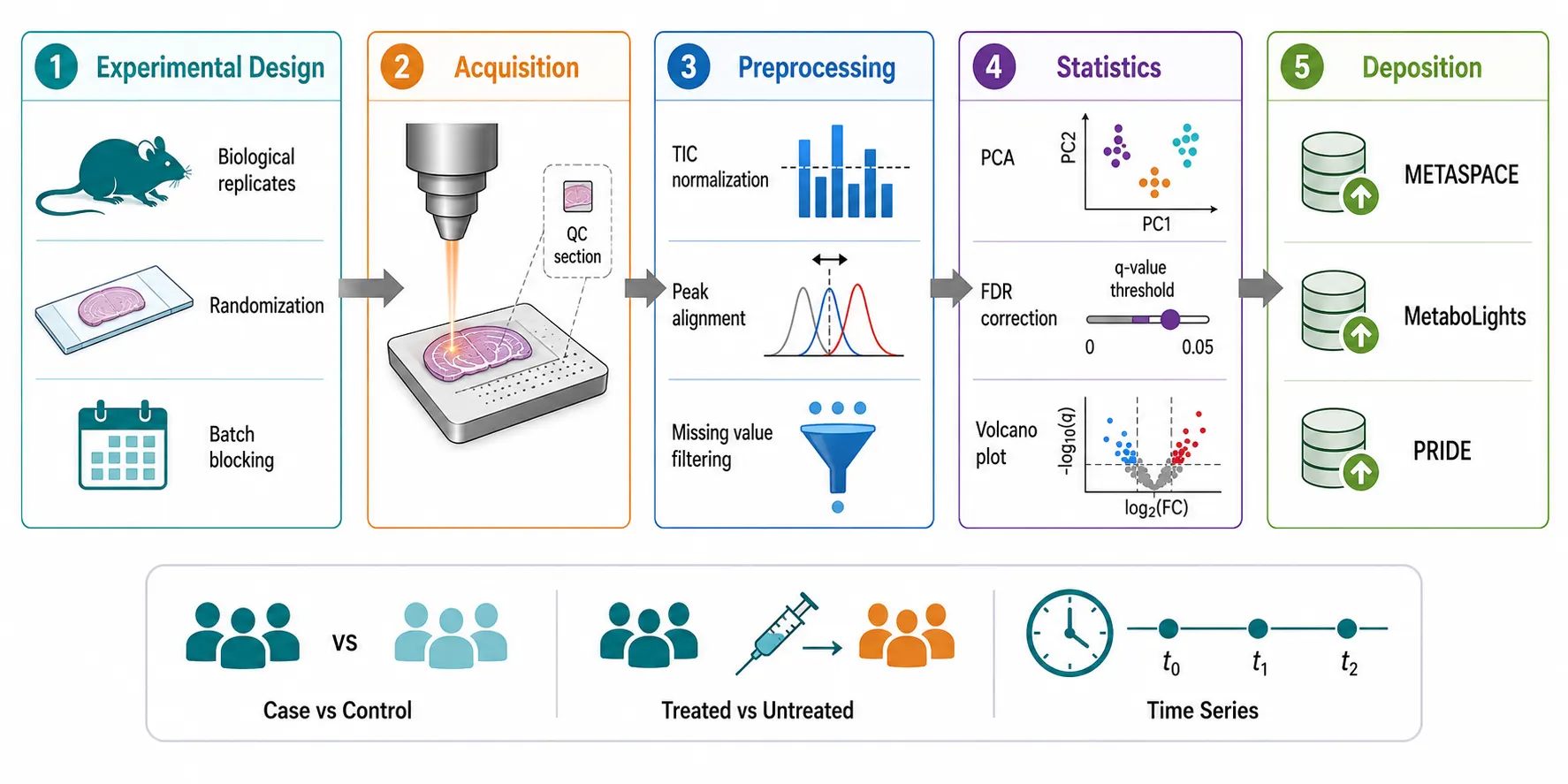 Figure 1: Comparative MSI Study Design — From Hypothesis to Multi-Group Statistical Testing. A horizontal workflow diagram illustrating the complete comparative MSI study pipeline across six stages: (1) Biological question formulation — clearly defining the comparison (case vs. control, treated vs. untreated, time series) and the expected spatial scale of metabolic differences; (2) Experimental unit determination — distinguishing the biological replicate (animal/tissue donor) from the observational unit (pixel), with a decision panel showing pixel-level, ROI-level, and subject-level aggregation strategies; (3) Group definition and sample size — N=3-5 biological replicates per group as the baseline, with randomization and blocking by slide; (4) MSI acquisition — block-randomized slide layout with QC sections at batch start and end; (5) Preprocessing — TIC/median normalization, peak alignment across sections, missing value imputation; (6) Statistical testing — univariate (t-test/ANOVA), multivariate (PCA/OPLS-DA), and spatial statistics with FDR correction. Each stage is rendered as a rounded rectangle with an icon, connected by directional arrows in a left-to-right flow on a clean white background.
Biological Replicate Requirements
A minimum of three to five biological replicates per group is the widely accepted baseline for comparative MSI studies, with the caveat that higher biological variability (common in patient-derived tissues) requires larger numbers. Phapale (2026) reinforces that biological replication must be addressed at the design stage, not treated as an afterthought once technical variability is observed. Technical replicates — repeat sections from the same tissue block — capture sectioning and acquisition variation but cannot substitute for biological replication. Underpowered studies risk both false negatives (missing true differences) and false positives (random clustering of technical artifacts masquerading as group separation in PCA scores plots).
Within-Subject vs. Between-Subject Designs
Within-subject designs, where a treated and control tissue region exist on the same slide (e.g., contralateral hemisphere of brain, or drug-treated vs. vehicle-treated flank tumor in the same animal), are statistically attractive because they eliminate inter-subject variability. Between-subject designs are unavoidable when the comparison cannot be housed in a single animal — for example, knockout vs. wild-type mice — and require careful attention to randomization and batch blocking.
Section Selection Strategy; Randomization and Blocking
Tissue sections from different experimental groups must be randomized across slide positions and acquisition order. A common failure mode is running all control samples first, followed by all treatment samples; any instrumental drift over the acquisition run becomes confounded with the treatment effect. The preferred approach is to block by slide: place one section from each treatment group on the same slide, randomize slide position, and randomize the acquisition order of slides across the instrument run — principles that apply equally to the in situ PK/PD profiling workflow where drug-treated and vehicle-control tissues must be co-localized on the same slide to eliminate batch confounding.
Batch Effect Control: One Acquisition vs. Multiple Sessions
Balluff et al. (2021) identified five levels at which batch effects manifest in MALDI-MSI: pixel-level (matrix heterogeneity, ion suppression), section-level (cutting and storage variation), slide-level (same-day preparation and acquisition), time-level (day-to-day instrument drift), and location-level (multi-center variation). For single-acquisition studies, the primary concern is within-run drift, which can be monitored with a quality control (QC) standard section placed at the beginning, middle, and end of the acquisition queue. For multi-session studies spanning days or weeks, Huang et al. (2025) demonstrated that a tissue-mimicking QC standard (propranolol embedded in gelatin) can track longitudinal technical variation across MALDI imaging workflow runs, and that computational correction methods including ComBat, WaveICA, and NormAE substantially reduce batch effects in MALDI-MSI data.
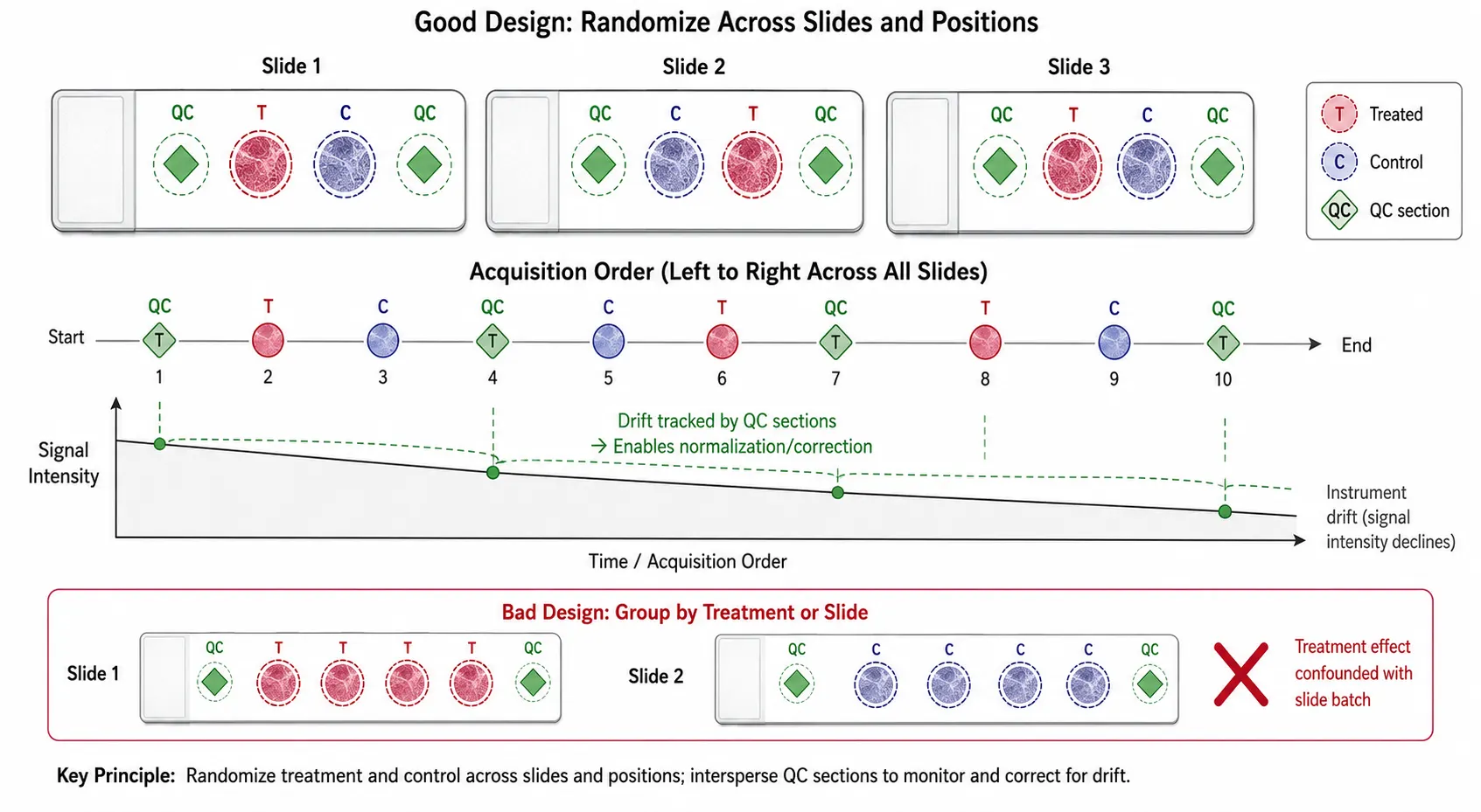 Figure 2: Five Levels of Batch Effects in MALDI-MSI and Randomization Strategy. A two-part infographic based on Balluff et al. (2021). Top panel — a concentric or stacked diagram illustrating the five hierarchical levels at which batch effects manifest in MALDI-MSI: (innermost) pixel-level — matrix heterogeneity and ion suppression within a single tissue section; section-level — cutting and storage variation between serial sections; slide-level — same-day preparation and acquisition effects; time-level — day-to-day instrument drift; (outermost) location-level — multi-center variation across laboratories. Each level is color-coded and annotated with the dominant source of variation and the recommended mitigation strategy. Bottom panel — a block-randomized slide layout schematic: a MALDI target plate with four groups (A, B, C, D) represented by colored squares, showing one section from each group placed on each slide in randomized positions, with a QC section at the start, middle, and end of the acquisition queue. A callout emphasizes the key design principle: "Randomize across slides, not within slides."
Cross-Section Normalization
After peak picking and alignment, the intensity of a given m/z feature must be comparable across tissue sections. Total ion current (TIC) normalization divides each pixel spectrum by its total ion count and is the most widely used method. Median normalization scales each spectrum to a common median intensity. Internal standard (IS)-based normalization, where a known compound is spiked into the matrix or applied as a spray coating, provides the most robust cross-section comparison when available. The choice of normalization method should be reported explicitly, as it directly affects downstream statistical results. For calibration and quantification protocols in MSI, see our guide on quantitative mass spectrometry imaging.
Peak Alignment Across Multiple Sections; Handling Missing Values
When spectra from multiple sections are combined into a single data matrix, the same metabolite must appear at the same m/z bin across all samples. Mass drift during acquisition causes peaks to shift by 10-50 ppm between sections, requiring alignment algorithms. Tools such as iMSminer (Python-based, GPU-accelerated) and Multi-MSIProcessor (Bi et al., 2024) provide dedicated cross-section peak alignment workflows. Missing values arise when a peak is detected in some sections but not others and must be handled by imputation or exclusion; common practice is to retain only m/z features present in at least 70-80% of samples within at least one group.
Quality Control Metrics for Multi-Sample MSI Studies
Huang et al. (2025) demonstrated that tracking the coefficient of variation (CV) of selected peaks in QC sections across the acquisition run provides a reliable indicator of technical variation. As a general benchmark, a median CV below 30% for QC peaks — consistent with FDA guidance for untargeted full-scan MS assays — is considered acceptable for comparative MSI studies. Principal component analysis (PCA) of all samples, colored by acquisition batch rather than experimental group, is a simple diagnostic: if batch explains more variance than biology, batch correction is necessary before group comparison.
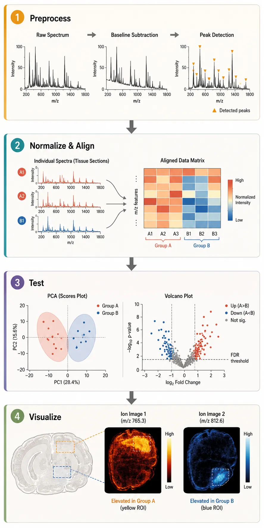 Figure 3: Cross-Section Normalization and Peak Alignment Pipeline. A five-stage horizontal pipeline diagram: (1) Raw multi-section MSI data ingestion — multiple tissue sections from different experimental groups shown as individual ion image thumbnails with visible intensity differences due to batch effects; (2) Normalization — a three-option panel comparing TIC normalization (dividing each pixel by total ion count), median normalization (scaling to common median intensity), and internal-standard-based normalization (spiked standard coating, most robust); (3) Peak alignment — mass drift correction visualized as overlapping extracted ion chromatograms before (offset peaks) and after (aligned peaks), with annotation of mass tolerance (10-50 ppm); (4) Missing value imputation — a feature matrix shown before (sparse, gaps) and after (filled), with the decision rule "retain m/z features present in ≥70-80% of samples in at least one group"; (5) Unified feature matrix output — a clean data matrix with samples as rows and m/z features as columns, annotated as "Ready for statistical testing." Software tools (iMSminer, Multi-MSIProcessor, Cardinal) are listed beneath their respective pipeline stages.
Univariate Testing: t-Test, ANOVA, Mann-Whitney per m/z
The most straightforward statistical approach is to perform a univariate test (t-test for two groups, ANOVA for three or more) on each m/z feature, using ROI-aggregated or subject-aggregated values as the input. Non-parametric alternatives (Mann-Whitney U, Kruskal-Wallis) are preferred when intensity distributions are non-normal, which is common in MSI data. The output is a list of m/z features ranked by p-value, which can be mapped back onto tissue coordinates to visualize spatially differential metabolites. Putative metabolite identifications from METASPACE or other annotation platforms can then be validated on a separate sample cohort using targeted metabolomics, confirming the identity and abundance of discriminant features.
Multiple Comparison Correction
With thousands of m/z features tested simultaneously, multiple comparison correction is essential. The Benjamini-Hochberg false discovery rate (FDR) procedure controls the expected proportion of false positives among declared discoveries. However, Cassese et al. (2016) demonstrated that standard FDR correction applied to pixel-wise tests (treating each pixel as independent) is anti-conservative because spatial autocorrelation inflates the effective number of tests. A spatial FDR approach — applying FDR correction to ROI-level or subject-level tests, or using spatially aware models — provides better error control.
Multivariate Methods: PCA, PLS-DA, OPLS-DA
Principal component analysis (PCA) is the workhorse for unsupervised exploration: it reveals whether groups separate naturally in the multivariate space and whether batch effects dominate biological signal. Partial least squares discriminant analysis (PLS-DA) and its orthogonal variant (OPLS-DA) are supervised methods that maximize group separation. OPLS-DA is widely used in MSI comparative studies because it separates class-discriminating variation from orthogonal (non-discriminating) variation, yielding clearer interpretability. For tissue lipid-focused comparative studies, MALDI-Imaging Lipidomics provides dedicated spatial lipid profiling with multivariate statistical support. Both methods require rigorous validation — permutation testing of the Q² statistic is the standard approach to verify that group separation is not a chance occurrence.
Spatial Statistics: Accounting for Spatial Autocorrelation
Cassese et al. (2016) showed that significant positive spatial autocorrelation (quantified by Moran's I) is present in all MALDI-MSI datasets and increases at higher spatial resolution — a statistical challenge that becomes even more acute at the single-cell level, where our single-cell spatial metabolomics guide addresses resolution-specific considerations for platforms operating below 5 μm pixel size. When pixels are spatially autocorrelated, classical tests treating pixels as independent produce inflated false positive rates. The authors demonstrated that conditional autoregressive (CAR) models accounting for spatial dependence reduce discovery rates by 21-69% compared to naive pixel-wise t-tests. In practice, the simplest mitigation is to aggregate pixels within ROIs before testing. More sophisticated approaches — CAR models, spatial generalized linear mixed models, and Moran's I-based filtering via packages such as SPUTNIK — are available for studies that require pixel-level inference.
ROI-Based vs. Pixel-Wise: When to Aggregate and When Not To
ROI-based aggregation is appropriate when the biological question concerns predefined anatomical compartments (e.g., tumor core vs. invasive margin vs. normal epithelium) and histological annotation is available. Pixel-wise analysis is necessary when the goal is to discover spatially restricted metabolic features without prior anatomical hypotheses — for example, identifying subregions of a tumor with distinct metabolic profiles that do not correspond to visible histological boundaries. The trade-off is interpretability vs. discovery power: ROI-based analysis is more statistically robust but may miss fine-grained spatial patterns, while pixel-wise analysis captures spatial detail at the cost of inflated false positive risk.
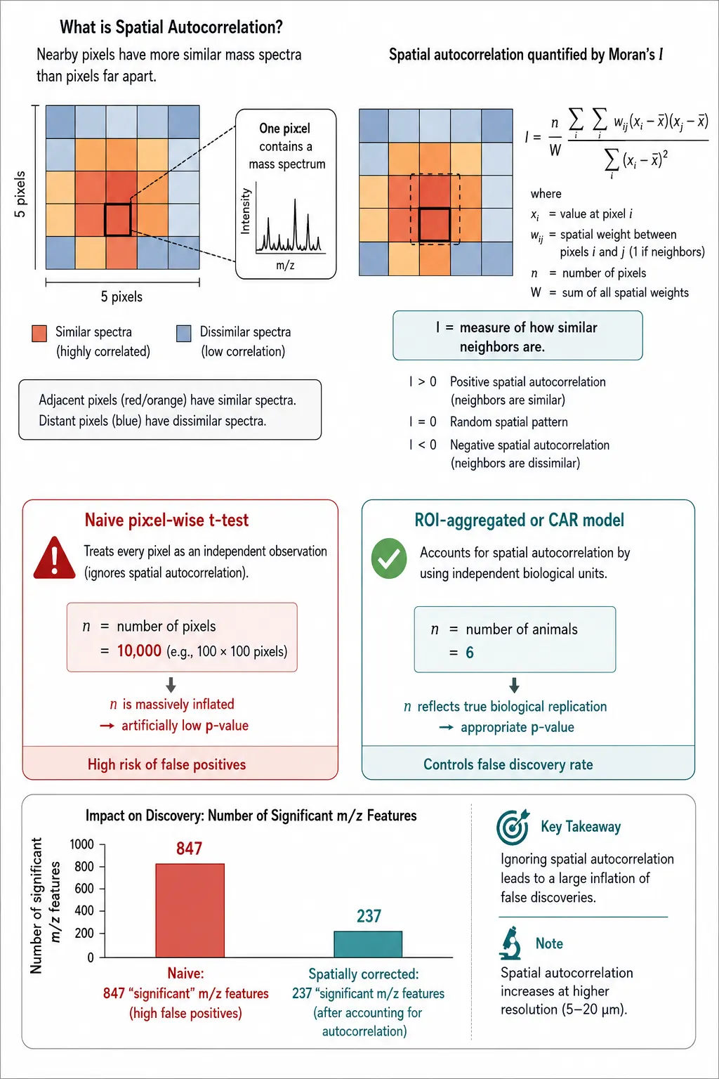 Figure 4: Spatial Statistics for MSI — Pixel-Wise vs. ROI-Based Testing with Multiple Comparison Correction. A side-by-side comparison infographic with three horizontal rows. Top row: the same tissue section displayed twice — left side shows pixel-level color coding (every pixel gets a test statistic), right side shows histologically annotated ROIs (tumor core, invasive margin, normal epithelium) as aggregated units. Middle row: statistical output comparison — left shows a volcano plot with thousands of points (pixel-wise tests) and a highlighted "spatial FDR" threshold line, annotated with "Inflated significance without spatial correction"; right shows a compact volcano plot with hundreds of points (ROI-aggregated tests), annotated with "Appropriate error control." Bottom row: a Moran's I correlogram showing spatial autocorrelation as a function of distance (high at short distances, decaying with lag) with a reference line at I=0 (no autocorrelation). A callout summarizes the Cassese et al. (2016) finding: spatial autocorrelation reduces effective sample size by 21-69% compared to naive pixel counting. Color palette: navy blue, teal accent, white background, clean modern academic infographic style.
Cardinal (R/Bioconductor), SCiLS Lab, METASPACE; Custom Python/R
Several software platforms support comparative MSI analysis. Cardinal (Bemis, Bioconductor v3.10.0, 2025) is an open-source R/Bioconductor package providing preprocessing, visualization, and statistical analysis of MSI data, with dedicated support for imzML format via CardinalIO. SCiLS Lab (Bruker) is a commercial platform offering spatial segmentation, PCA, PLS-DA, co-localization analysis, and multi-vendor data support through imzML import; its 2025 release emphasizes multiomics fusion and CCS-enabled metabolite annotation via MetaboScape integration. METASPACE (metaspace2020.eu) provides cloud-based FDR-controlled metabolite annotation and has recently added enrichment analysis capabilities. For custom workflows, iMSminer (Python) and SPUTNIK (R) offer specialized functionality for multi-condition peak alignment and spatial randomness filtering, respectively. For studies requiring pathway-level interpretation of spatially differential features, Bioinformatics for Metabolomics provides enrichment analysis and network mapping that contextualize MSI results within known metabolic pathways. The haCCA framework (Xu et al., 2026) extends comparative analysis to multi-modal integration, using canonical correlation analysis to identify correlated gene-metabolite features across spatial transcriptomics and MSI data.
Reporting Standards and Reproducibility
What to Report; Data Deposition
A comparative MSI study should report, at minimum: the number of biological and technical replicates per group; the randomization and blocking scheme; the normalization method; the peak alignment parameters; the statistical test used and the unit of analysis (pixel, ROI, or subject); and the multiple comparison correction method with the chosen FDR threshold. Raw data in imzML format and processed feature matrices should be deposited in public repositories. METASPACE accepts imaging MS datasets for FDR-controlled metabolite annotation and public sharing. MetaboLights and PRIDE (for proteomics-focused MSI) serve as general-purpose metabolomics and proteomics repositories, respectively.
Case Study Walkthrough
Worked Example: Tumor vs. Normal — From Raw Data to Interpretation
Consider a study comparing metabolite profiles of human colorectal tumor tissue vs. matched adjacent normal mucosa from six patients (n = 6 per group). Sections from each patient are randomized across two slides (three tumor and three normal per slide), with a QC section at the start and end of each slide. After MALDI-MSI acquisition, spectra are processed in Cardinal: TIC normalization, peak picking (signal-to-noise ratio > 5), and peak alignment across all 12 sections. A PCA scores plot colored by patient reveals that patient identity explains more variance than tissue type, confirming the need for a paired analysis. For each m/z feature, a paired t-test is performed on ROI-averaged intensities (tumor ROI vs. normal ROI per patient). Benjamini-Hochberg FDR correction is applied across all tested m/z features. Features with FDR < 0.05 and fold change > 1.5 are annotated via METASPACE against the CoreMetabolome database. In practice, a substantial fraction of the differentially abundant ions in tumor-vs-normal comparisons are lipids, making MALDI-Imaging Lipidomics a particularly relevant analytical strategy for cancer metabolism studies. The resulting set of differential metabolites — elevated in tumor or depleted in tumor — is visualized as a volcano plot and as annotated ion images showing spatial localization.
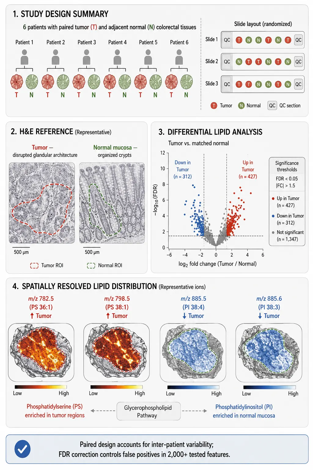 Figure 5: Comparative MSI Data Analysis Pipeline — From Raw Spectra to Biological Insight. A comprehensive five-stage vertical workflow with representative data outputs at each stage. Stage 1: Multi-sample raw MSI data — a grid of ion image thumbnails from individual tissue sections, with experimental group labels (Tumor, Normal) and batch ID. Stage 2: Preprocessing — a panel showing TIC normalization (before/after intensity distribution histograms), peak picking (S/N > 5 threshold), and a PCA scores plot colored by acquisition batch (diagnostic for batch effects). Stage 3: Peak alignment and feature matrix — a heatmap visualization of the aligned feature matrix with hierarchical clustering dendrograms on both axes, showing group separation. Stage 4: Statistical testing — a volcano plot (log2 fold change vs. -log10 p-value) with FDR < 0.05 threshold line, significantly differential features highlighted in teal, alongside a spatial projection showing the tissue distribution of the top 3 differential features. Stage 5: Biological interpretation — METASPACE metabolite annotation results displayed as a bar chart of identified compounds, connected to a KEGG pathway map with differential metabolites highlighted. Software platforms (Cardinal, SCiLS Lab, METASPACE, iMSminer) and statistical methods (t-test, OPLS-DA, CAR models) are listed beside their respective stages.
FAQ
Q: How many biological replicates do I need for a comparative MSI study?
A: A minimum of three to five biological replicates per group is the general recommendation, but higher biological variability (e.g., patient-derived tissues) calls for larger sample sizes. Technical replicates (repeat sections from the same block) can help estimate technical variance but do not substitute for independent biological samples.
Q: Should I use pixel-wise or ROI-based statistical testing?
A: Use ROI-based testing when your question concerns predefined anatomical compartments and histological annotation is available. Use pixel-wise testing for discovery of spatially restricted features, but account for spatial autocorrelation via appropriate models (e.g., CAR models) and be aware that standard p-values will be anti-conservative.
Q: My PCA shows separation by acquisition batch instead of biological group. What should I do?
A: This indicates batch effects are dominating biological signal. Apply computational batch correction (ComBat, WaveICA, or NormAE) and include QC sections in your acquisition design. Huang et al. (2025) provide a practical workflow for evaluating and correcting batch effects.
Q: Can I combine MSI data with other spatial modalities in a comparative study?
A: Yes. The haCCA framework (Xu et al., 2026) integrates MALDI-MSI metabolomics with spatial transcriptomics using canonical correlation analysis, complementing integrated proteomics and metabolomics analysis workflows, enabling identification of correlated gene-metabolite spatial features. This approach requires co-registration of the two data modalities to a common coordinate system.
Q: Where should I deposit my comparative MSI data for publication?
A: METASPACE is the primary repository for imaging MS-based metabolomics data and provides FDR-controlled annotation. MetaboLights accepts general metabolomics datasets including MSI. For multi-omics studies incorporating MS-based Spatial Proteomics, PRIDE is appropriate for the proteomics component.
References:
- Phapale P. Spatial metabolomics: design, pitfalls and data interpretation. EMBO J. 2026;45(19):4007-4013. doi:10.1038/s44318-026-00797-x
- Balluff B, Hopf C, Porta Siegel T, Grabsch HI, Heeren RMA. Batch effects in MALDI mass spectrometry imaging. J Am Soc Mass Spectrom. 2021;32(3):628-635. doi:10.1021/jasms.0c00393
- Huang L, Kim Y, Balluff B, Cillero-Pastor B. Quality control standards for batch effect evaluation and correction in mass spectrometry imaging. Anal Chem. 2025;97(20):10919-10928. doi:10.1021/acs.analchem.5c02020
- Cassese A, Ellis SR, Ogrinc Potočnik N, Heeren RMA, et al. Spatial autocorrelation in mass spectrometry imaging. Anal Chem. 2016;88(11):5871-5878. doi:10.1021/acs.analchem.6b00672
- Xu J, Shen XT, Zhang C, Zhang XY, Chen ZQ, Jia HL, Yang LY. haCCA: multi-module integration of spot-based spatial transcriptomes and metabolomes. Commun Biol. 2026;9(1):1. doi:10.1038/s42003-026-09526-w
- Bi S, Wang M, Pu Q, Yang J, Jiang N, Zhao X, Qiu S, Liu R, Xu R, Li X, Hu C, Yang L, Gu J, Du D. Multi-MSIProcessor: data visualizing and analysis software for spatial metabolomics research. Anal Chem. 2024;96(1):339-346. doi:10.1021/acs.analchem.3c04192