A laboratory director evaluating a $60,000–120,000 instrument upgrade faces a decision that ties together capital expenditure, method validation timelines, operator training, and long-term consumables cost. The question is not simply whether UHPLC outperforms HPLC –it is whether the performance differential translates to a measurable return within your specific analytical workflow. This article goes beyond the surface-level comparison of particle sizes and pressure ratings to examine the chromatographic theory that dictates real-world performance differences, walk through the practical mathematics of method transfer, address the often-overlooked variables that can sabotage a UHPLC implementation, and provide a decision framework calibrated to analytical goals rather than instrument specifications. For further reading on this topic, see our dedicated resource on lc-ms vs lc-ms/ms.
HPLC-based analysis services provide method development, optimization, and routine analysis across diverse sample types in proteomics and metabolomics workflows.
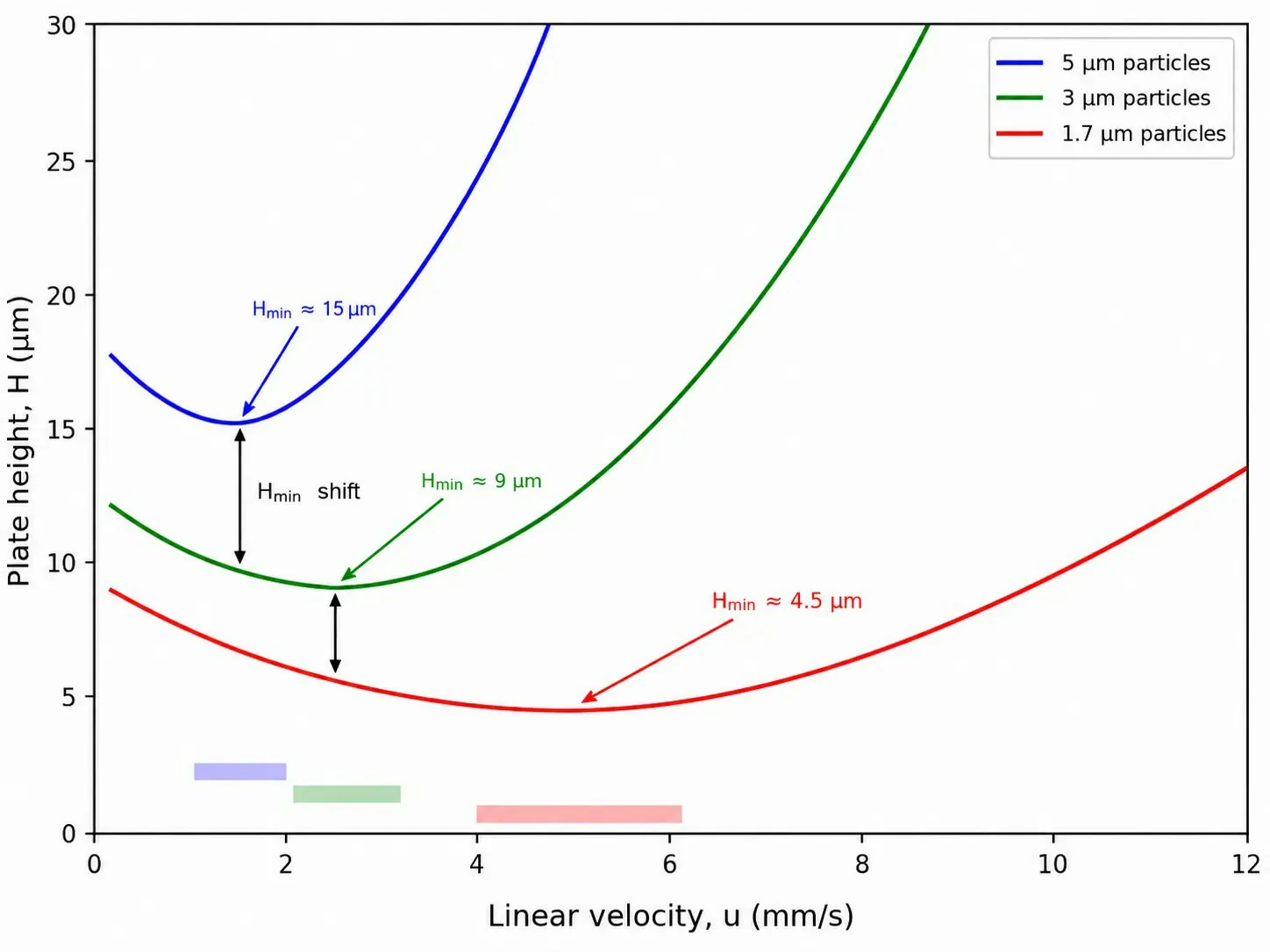
Figure 1: Van Deemter curves for 5 μm, 3 μm, and sub-2 μm fully porous particles, plotted as plate height (H) vs. linear velocity (u), with optimal velocity ranges annotated and the shift in H_min highlighted
The Theoretical Foundation: Why Particle Size Dictates Performance
The performance gap between HPLC and UHPLC originates not in pump engineering or detector design, but in a single physical parameter: stationary phase particle diameter (dp). Understanding why requires examining the Van Deemter equation, which relates plate height (H) –a measure of band broadening inversely proportional to column efficiency –to mobile phase linear velocity (u).
The Van Deemter Equation in Practice
The simplified Van Deemter equation is expressed as:
H = A + B/u + C·u
Each term corresponds to a distinct band-broadening mechanism:
The A-term (eddy diffusion) accounts for the multiple flow paths a solute molecule can take through a packed bed. Smaller particles produce a more homogeneous packing structure, reducing the path-length variability that causes band dispersion. For a well-packed 5 μm column, A typically contributes 10–15 μm to plate height; for a sub-2 μm column, this drops below 5 μm. The practical consequence is narrower peaks and higher resolution per unit column length. The A-term is proportional to particle diameter and depends critically on packing quality –poorly packed UHPLC columns lose much of the theoretical advantage predicted by particle size alone.
The B-term (longitudinal diffusion) describes axial molecular diffusion along the column axis. This term is inversely proportional to linear velocity because slower flow allows more time for diffusion-driven band spreading. The B-term is largely independent of particle size –it depends on the solute diffusion coefficient in the mobile phase. At the optimal linear velocity, B-term contributions are modest for both HPLC and UHPLC, contributing less than 10% of total plate height in well-optimized methods.
The C-term (mass transfer resistance) is where UHPLC achieves its decisive advantage. This term quantifies the resistance to solute equilibration between the mobile phase and the stationary phase within the pores. Smaller particles shorten the diffusion path length into and out of the pore structure, dramatically reducing the C-term coefficient. The C-term scales with dp², meaning the reduction from 5 μm to 1.7 μm particles is approximately ninefold. For a 5 μm fully porous particle, the characteristic diffusion distance is ~2.5 μm (the particle radius); for a 1.7 μm particle, it is ~0.85 μm –three times shorter, yielding dramatically improved mass transfer kinetics.
From Theory to Chromatographic Reality
The critical insight from the Van Deemter curve is that the optimal linear velocity shifts to higher values as particle size decreases. A conventional 5 μm column achieves minimum plate height at approximately 1–2 mm/s, whereas a 1.7 μm column reaches its minimum at 4–6 mm/s –and the curve is flatter beyond the minimum. This means UHPLC can operate at significantly higher flow rates without the efficiency penalty that would cripple an HPLC column. The combination of higher optimal velocity and shorter column length (50–100 mm for UHPLC vs. 150–250 mm for HPLC) explains the order-of-magnitude reduction in analysis time while maintaining or exceeding total plate count. For a laboratory optimizing an LC-MS analysis workflow, understanding these theoretical relationships is essential for intelligent method development rather than trial-and-error parameter adjustment.
Critical Performance Parameters: A Quantitative Comparison
Resolution and Peak Capacity
Resolution (Rs) between adjacent peaks is governed by three factors captured in the fundamental resolution equation: efficiency (N), selectivity (α), and retention factor (k). UHPLC primarily improves the efficiency term. A 100 mm column packed with 1.7 μm particles can deliver 15,000–20,000 theoretical plates –comparable to a 250 mm column packed with 5 μm particles –but does so in approximately one-third to one-fifth of the analysis time. Peak capacity, which describes the maximum number of peaks resolvable in a given gradient window, increases with the square root of plate count, such that nc ≅ 1 + (√N/4) · ln(1 + kf). For typical gradient separations, UHPLC peak capacities of 300–500 are routinely achievable, compared to 150–250 for optimized HPLC methods.
The practical implication for complex sample analysis –metabolomics extracts, proteolytic digests, natural product fractions –is substantial. Two co-eluting peaks that merge into a single unresolved feature on an HPLC system can often be baseline-resolved on UHPLC without any change to mobile phase chemistry. In untargeted metabolomics applications, where thousands of features must be distinguished in a single run, the peak capacity difference between HPLC and UHPLC directly determines how many metabolites can be reliably identified and quantified.
Sensitivity and Limit of Detection
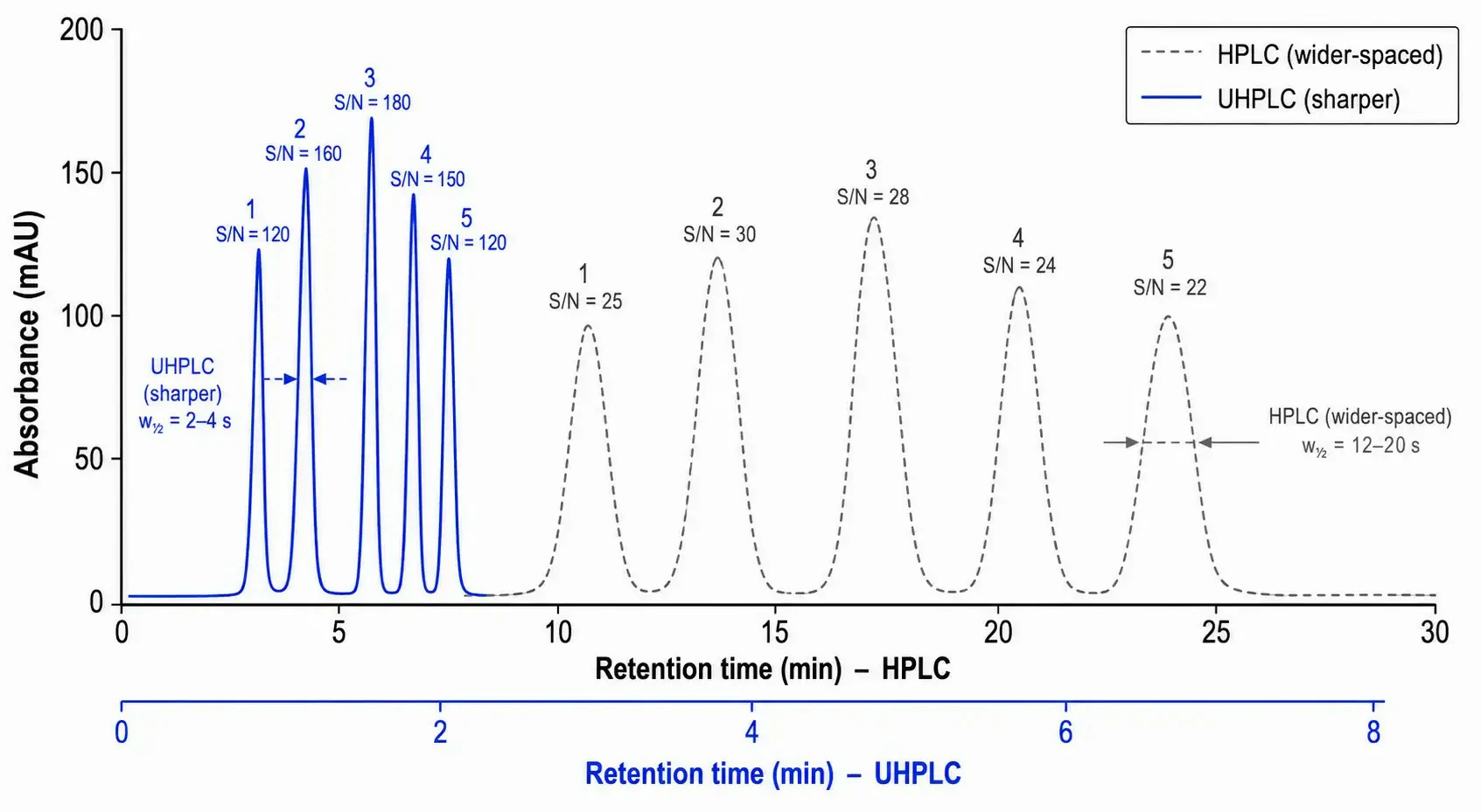
UHPLC generates narrower peaks –typically 2–5 seconds at baseline width vs. 10–30 seconds for HPLC –which concentrates the analyte mass into a smaller elution volume. For a concentration-sensitive detector such as UV-Vis, this translates directly to higher peak height and improved signal-to-noise ratio (S/N). Empirical comparisons show S/N improvements of 3- to 10-fold when transferring an HPLC method to UHPLC under geometrically scaled conditions. For mass spectrometry detection, the sharper peaks increase the number of data points across each peak –essential for accurate quantitation in selected reaction monitoring (SRM) and parallel reaction monitoring (PRM) workflows. In targeted metabolomics, this translates to lower limits of quantification (LOQ) and more confident peak integration for low-abundance analytes in complex biological matrices.
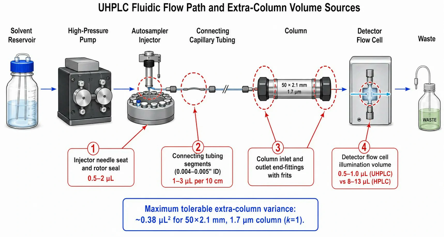
However, this sensitivity gain is contingent on detector flow cell design. UHPLC demands smaller illumination volumes –typically 0.5–1.0 μL vs. 8–13 μL for conventional HPLC –to avoid re-mixing of resolved peaks within the detector itself. Laboratories retrofitting older detectors to UHPLC systems unknowingly sacrifice the resolution they paid for, because the large detector cell volume negates the narrow peak widths produced by the column.
Figure 2: Overlay of chromatograms for a five-component test mixture separated on a 150 × 4.6 mm, 5 μm HPLC column vs. a 50 × 2.1 mm, 1.7 μm UHPLC column, with retention times, peak widths at half-height (w½), and S/N values annotated for key peaks
Analysis Speed and Throughput
Reducing column dimensions from 150 × 4.6 mm to 50 × 2.1 mm –a typical geometric scaling for method transfer –decreases the column void volume from approximately 1.5 mL to 0.12 mL. At equivalent reduced linear velocity, this translates to gradient times of 2–5 minutes for UHPLC vs. 15–30 minutes for HPLC. For high-throughput environments processing hundreds of samples per week, the throughput gain enables laboratories to complete analytical campaigns in days rather than weeks. The solvent consumption reduction –from 1.2–1.5 L per 10-hour run on HPLC to approximately 250 mL on UHPLC –generates ongoing operational savings that compound over the instrument lifetime.
Instrument Architecture: What Changes Under the Hood
Pumping Systems and Pressure Tolerance
Modern UHPLC pumping systems must deliver pulse-free flow at pressures exceeding 15,000 psi (approximately 1,000 bar), compared to the 6,000 psi ceiling of conventional HPLC pumps. This requires binary or quaternary pump designs with low-pressure gradient formation, specialized check valves rated for high-pressure operation, and high-pressure mixing chambers engineered for minimal gradient delay volume. Pump seals and pistons in UHPLC systems experience accelerated wear due to the combination of high pressure and rapid piston stroke cycles –a practical consideration often underappreciated by laboratories transitioning from HPLC. Preventive maintenance intervals for UHPLC pump seals are typically every 6–12 months under continuous use, approximately half the interval expected for HPLC pumps.
The solvent compressibility problem intensifies at UHPLC pressures. Mobile phases are not perfectly incompressible; at 1,000 bar, methanol compresses by approximately 4% and acetonitrile by roughly 8% relative to their volumes at atmospheric pressure. Modern UHPLC pumps incorporate compressibility compensation algorithms that pre-compress each solvent before the pump stroke delivers it to the mixer, maintaining accurate flow rates. However, these algorithms are solvent-specific and may require recalibration when switching between significantly different mobile phase compositions, particularly for gradient methods spanning a wide organic-to-aqueous range.
Column Technology: Particle Morphology Matters
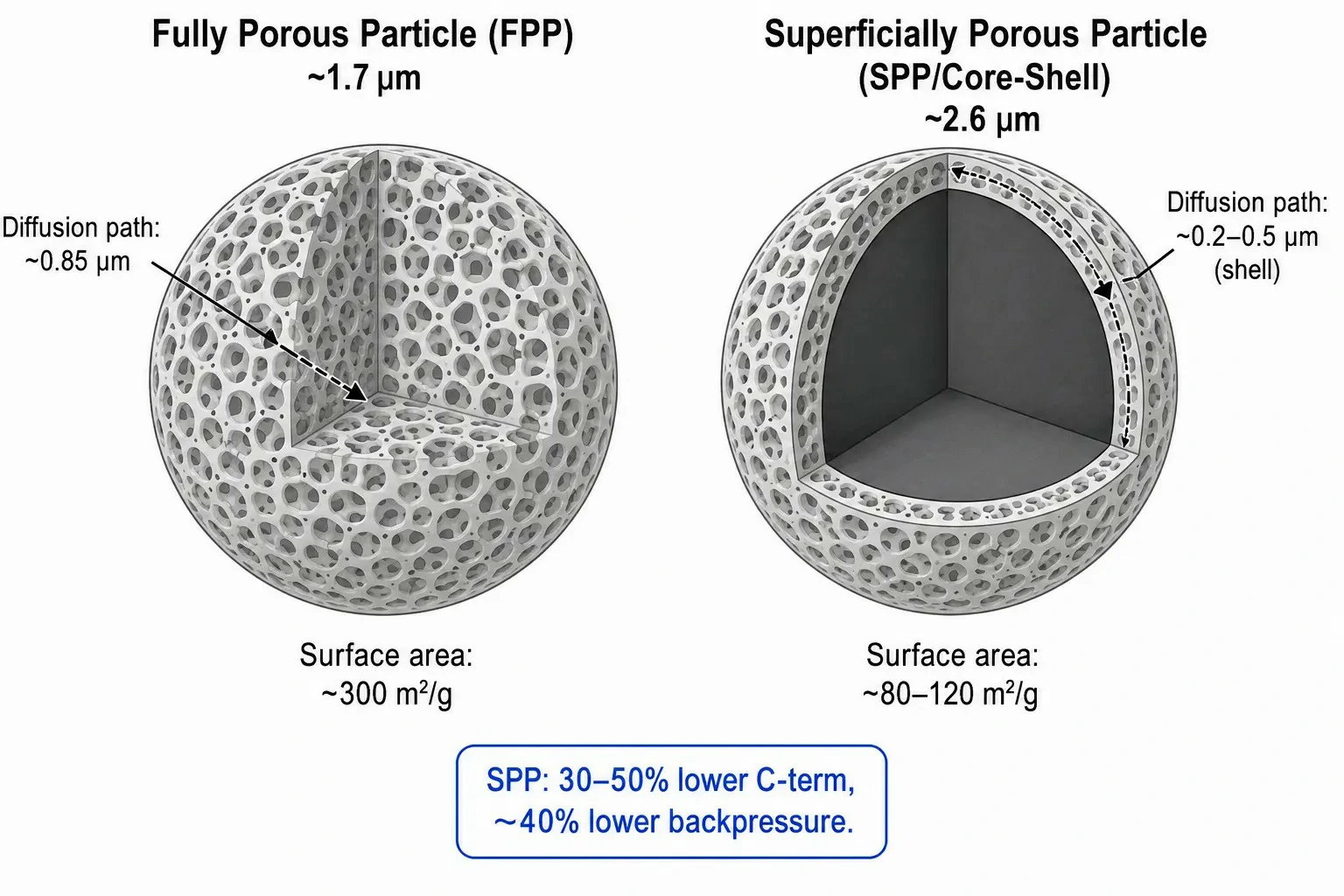
Beyond particle size, particle morphology exerts a profound influence on chromatographic performance. Fully porous particles (FPPs) –the traditional standard for both HPLC and UHPLC –provide high surface area (~300 m²/g for a 1.7 μm C18 material) and correspondingly high loading capacity. However, the diffusion path length through the entire porous structure limits mass transfer kinetics, as described by the C-term. For a 1.7 μm FPP, solute molecules must diffuse approximately 0.85 μm into and out of the pore network to equilibrate between the mobile and stationary phases.
Superficially porous particles (SPPs), also known as core-shell or fused-core particles, consist of a solid, non-porous silica core surrounded by a thin porous shell of 0.2–0.5 μm thickness. This architecture reduces the diffusion distance to the shell thickness rather than the full particle radius, cutting the effective C-term by an additional 30–50% compared to equivalent-size FPPs. The result is comparable or superior efficiency at a given particle size –but with approximately 25–40% lower backpressure, because the larger solid core means the interstitial channels between particles are wider at the same particle diameter. This lower backpressure allows SPP-based columns (e.g., 2.6–2.7 μm superficially porous) to achieve near-UHPLC performance on HPLC systems rated to 6,000–9,000 psi –a practical bridge technology for laboratories not ready to commit to a full UHPLC platform.
The tradeoff is loading capacity: SPPs have roughly 25–40% of the accessible surface area of equivalent-size FPPs, making them less suitable for preparative-scale separations or trace-enrichment applications where binding capacity is paramount. For analytical-scale work at typical injection masses of 1–100 ng per component, this capacity difference is rarely limiting. Selecting between FPP and SPP columns depends on the analytical priority: maximum absolute efficiency at the highest pressure (FPP sub-2 μm) vs. near-UHPLC performance on moderate-pressure systems with lower cost of ownership (SPP 2.6–2.7 μm).
Figure 3: Cross-sectional schematic comparing fully porous particle (FPP) and superficially porous particle (SPP/core-shell) architectures, with effective diffusion path lengths and surface area values annotated for each particle type
The Extra-Column Volume Problem
Perhaps the most insidious source of performance degradation in UHPLC is extra-column band broadening –dispersion occurring outside the column, in the injector, connecting tubing, and detector flow cell. Because UHPLC peaks elute in volumes of 10–20 μL (compared to 100–200 μL for HPLC), any unswept volume in the flow path contributes disproportionately to peak broadening.
The total extra-column variance (σ²ec) should not exceed 10% of the column variance for the earliest-eluting peak of interest. For a 50 × 2.1 mm, 1.7 μm column with a void volume of approximately 120 μL and a plate count of 15,000, the column variance for k = 1 is σ²col = (V0·(1 + k)/√N)² ≅ (120 × 2 / 122.5)² ≅ 3.8 μL². The maximum tolerable extra-column variance is therefore 0.38 μL², corresponding to a maximum extra-column volume of approximately 5–8 μL. Standard HPLC stainless steel tubing with 0.010" or 0.020" internal diameter introduces unacceptable dead volume; UHPLC systems use 0.004–0.005" ID tubing with zero-dead-volume fittings throughout the entire flow path from injector to detector.
Laboratories that attempt to pair a UHPLC column with an HPLC autosampler and detector frequently observe peak widths 30–50% broader than the column's theoretical performance –not because the column is defective, but because the system dispersion erodes the separation before it reaches the detector. A systematic audit of extra-column volume sources –injector needle seat, all tubing segments, column inlet and outlet frits, and detector flow cell –is an essential step when commissioning a new UHPLC system or troubleshooting unexpectedly poor peak shape.
Figure 4: Schematic of a UHPLC flow path identifying extra-column volume sources –injector needle seat, connecting tubing segments, column end-fittings, and detector flow cell –with typical dispersion contribution values and acceptable limits annotated
Method Transfer: Bridging HPLC and UHPLC
Geometric Scaling: The Mathematical Framework
Transferring an isocratic method from HPLC to UHPLC follows a geometric scaling framework that preserves the reduced linear velocity and the number of column volumes passed during the separation. The key scaling relationships are derived from the requirement that the separation environment –reduced velocity (ν), reduced plate height (h), and gradient steepness parameter (b) –remains constant between platforms.
Flow rate scaling: F₂ = F₁ × (dc₂²/dc₁²) × (dp₁/dp₂), where dc is column internal diameter and dp is particle size. For a transfer from 150 × 4.6 mm, 5 μm to 50 × 2.1 mm, 1.7 μm: F₂ = F₁ × (2.1²/4.6²) × (5.0/1.7) ≅ F₁ × 0.208 × 2.94 ≅ 0.61 × F₁. If the original HPLC method ran at 1.0 mL/min, the geometrically equivalent UHPLC flow rate is approximately 0.6 mL/min.
Injection volume scaling: V₂ = V₁ × (dc₂² × L₂) / (dc₁² × L₁). Using the same column dimensions: V₂ = V₁ × (2.1² × 50) / (4.6² × 150) ≅ V₁ × 0.069. A 10 μL HPLC injection scales to approximately 0.7 μL on UHPLC. This drastic reduction in injection volume is essential to prevent mass overload of the smaller column and to maintain the narrower peak widths that UHPLC is designed to produce.
Gradient time scaling: For gradient methods, the gradient steepness parameter (b) must be preserved: tG₂ = tG₁ × (F₁/F₂) × (Vm₂/Vm₁), where Vm is the column void volume approximated by Vm ≅ 0.68 × L × dc² × π/4. A 30-minute HPLC gradient typically scales to a 4–6 minute UHPLC gradient, providing the dramatic throughput increase that justifies the platform investment for many laboratories.
Gradient Dwell Volume: The Hidden Variable
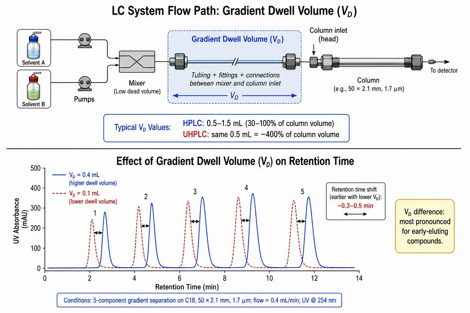
Geometric scaling assumes that the gradient formed by the pump reaches the column inlet at the programmed time. In reality, every HPLC/UHPLC system has a gradient dwell volume (VD) –the physical volume between the point of gradient mixing and the column head. This includes the mixer chamber, connecting capillary tubing, autosampler metering device and loop, and injection valve internal passages.
For HPLC, a VD of 0.5–1.5 mL is typical and represents roughly 30–100% of the column void volume of a 150 × 4.6 mm column –significant, but manageable with an isocratic hold programmed at the start of the gradient. For UHPLC, the same absolute dwell volume of 0.5 mL represents approximately 400% of the column void volume of a 50 × 2.1 mm column. The consequence is an extended isocratic hold at the gradient start that the chromatographer did not program, altering the effective gradient profile at the column inlet and shifting retention times systematically. Compounds eluting early in the gradient are most affected, because the isocratic segment consumes a larger fraction of their total migration time.
When transferring a method between UHPLC systems from different manufacturers –or even between different models from the same manufacturer –dwell volume differences are the most common cause of irreproducible retention times. A systematic strategy involves measuring the actual dwell volume of both source and destination systems using a zero-dead-volume union in place of the column and a step-gradient of UV-absorbing tracer, then applying a gradient delay correction equal to (VDest − VOrig) / FDest in the method program.
Figure 5: Schematic illustrating gradient dwell volume –the physical volume between the gradient mixer and the column head –with overlaid chromatograms demonstrating the effect of a 0.4 mL vs. 0.1 mL dwell volume difference on retention times for a five-component gradient separation
Practical Transfer Protocol
A robust HPLC-to-UHPLC method transfer proceeds in four systematic steps:
Step 1 –Dwell Volume Measurement: Replace the column with a zero-dead-volume union. Run a step gradient of 0.1% acetone (or uracil) in mobile phase A to 100% B, monitoring absorbance at 254–265 nm. The time from the start of the gradient program to the midpoint of the absorbance rise, multiplied by the flow rate, equals the system dwell volume. Repeat three times and use the mean value.
Step 2 –Geometric Scaling Calculation: Apply the flow rate, injection volume, and gradient time scaling equations described above. Use actual (measured) column dimensions and particle sizes rather than nominal values whenever possible.
Step 3 –Dwell Volume Correction: Insert an isocratic hold at the gradient start on the destination system equal to (VDest − VOrig) / FDest. This ensures the gradient arrives at the column at the same elution strength and time relative to column volumes as in the original method.
Step 4 –Validation: Inject a system suitability test mixture on both platforms. Acceptance criteria: retention time deviation ≤ 5% for all peaks, resolution (Rs) not reduced by more than 10% from the original method, and peak asymmetry (As) ≤ 1.5 for the critical pair. If acceptance criteria are not met, verify extra-column volume, check column temperature control accuracy, and recalibrate the dwell volume measurement.
For laboratories outsourcing method development, customized analytical method development services can perform the scaling calculation, transfer, and validation, delivering a fully qualified UHPLC method with documented system suitability criteria.
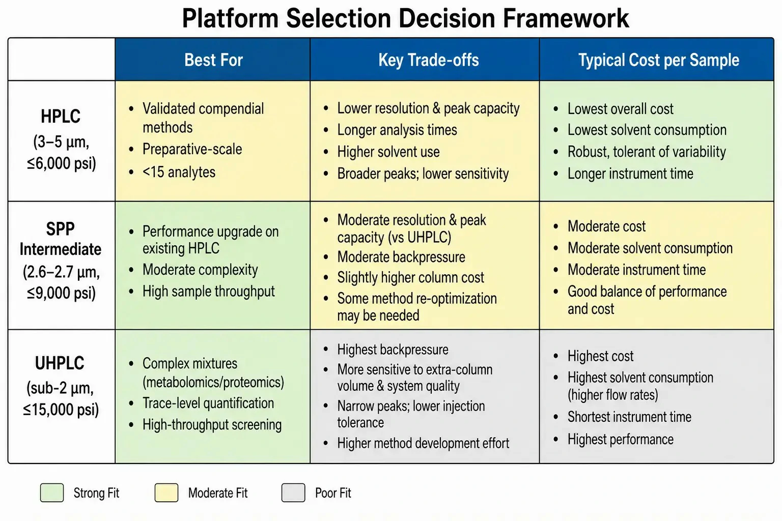
Figure 6: Decision matrix mapping common analytical objectives (QC release testing, R&D impurity profiling, trace-level quantification, high-throughput screening, complex mixture characterization) to the recommended platform (HPLC, UHPLC, or SPP-based intermediate), with the primary decision drivers annotated
Decision Framework: Which Platform for Which Analytical Goal
The optimal platform is not a function of superior specifications in isolation but of alignment between instrument capability and analytical objectives. The following framework maps common laboratory scenarios to a platform recommendation based on operational variables that actually drive return on investment.
HPLC remains the rational choice when: The analytical workflow is built around validated, compendial methods that would require revalidation if transferred. QC release testing in regulated environments –where method robustness, long-term reproducibility, and operator familiarity outweigh incremental speed gains –is the canonical HPLC stronghold. HPLC also serves laboratories running preparative-scale separations, where the higher loading capacity of larger-diameter columns (10–21 mm ID) and the lower cost of larger-particle stationary phases (5–10 μm) are essential. Additionally, laboratories analyzing simple mixtures with fewer than 10–15 components of interest rarely benefit from UHPLC peak capacity; a well-optimized HPLC method with 8,000–10,000 plates is more than sufficient, and the instrument capital can be directed toward sample preparation automation or additional detectors.
UHPLC becomes the preferred platform when: Sample complexity exceeds the peak capacity of optimized HPLC –typical of metabolomics, lipidomics, and proteomics applications where hundreds to thousands of features must be distinguished. High-throughput requirements, where instrument time rather than method development time is the rate-limiting step, also favor UHPLC: a method delivering equivalent resolution in 5 minutes rather than 25 minutes increases daily sample capacity fivefold. Trace-level quantification demanding the highest possible S/N –residue analysis, impurity profiling at the 0.05% threshold, biomarker verification in limited-volume biofluids –benefits directly from the narrower peak widths and higher sensitivity of UHPLC-MS. Metabolomics analysis services leverage UHPLC-MS platforms to achieve the peak capacity and sensitivity required for comprehensive metabolite profiling.
SPP-based intermediate systems (2.6–2.7 μm superficially porous particles on moderate-pressure instruments rated to 6,000–9,000 psi) represent a practical compromise: they deliver approximately 70–80% of the efficiency gain of sub-2 μm UHPLC but at 40–50% of the backpressure, enabling operation on HPLC-class pumps. This approach is particularly well-suited for laboratories that need improved performance but cannot justify the full capital outlay for a dedicated UHPLC system, or for methods where loading capacity requirements preclude the smaller column dimensions typical of sub-2 μm UHPLC.
Conclusion
The HPLC vs. UHPLC decision is fundamentally a question of whether the analytical workflow justifies the investment in higher pressure, smaller particles, and stricter system requirements. UHPLC delivers unequivocally superior chromatographic performance –higher resolution, greater sensitivity, and dramatically faster analysis times –but only when the laboratory's sample complexity, throughput demands, and detection requirements create a genuine need for this additional capability. The theoretical foundation, grounded in the Van Deemter equation and mass transfer kinetics, explains why these performance gains occur; the practical considerations of extra-column volume, gradient dwell volume, and particle morphology determine whether those gains are realized in daily operation. Method transfer between platforms, while mathematically straightforward through geometric scaling, demands attention to dwell volume differences that can silently erode reproducibility. By aligning platform selection with analytical objectives –rather than chasing specifications –laboratories can allocate instrumentation budgets to maximum effect.
For laboratories processing complex mixtures, running high-throughput batches, or performing trace-level quantification, UHPLC delivers a measurable return on investment through reduced instrument time –often 4–9× faster per run –lower per-sample solvent costs, and improved data quality from narrower, more intense peaks. Laboratories operating validated compendial methods or preparative-scale workflows will find that a well-optimized HPLC system, or an SPP-based intermediate upgrade on moderate-pressure instrumentation, provides the more capital-efficient path. This preserves budget for orthogonal investments such as sample preparation automation, additional detectors, or laboratory information management system (LIMS) integration that can yield comparable workflow improvements at lower instrument cost.
Frequently Asked Questions
Can I use my HPLC columns on a UHPLC system?
HPLC columns with 3–5 μm particles can be operated on a UHPLC system, but the pressure generated at typical UHPLC flow rates will be far lower than what the UHPLC pump is designed to deliver. More importantly, the large internal diameter of standard HPLC columns (4.6 mm) combined with the UHPLC system's optimized low-dispersion flow path means the extra-column volume contribution to peak width is negligible –providing a modest efficiency benefit even with HPLC columns. However, HPLC columns do not exploit the full capability of the UHPLC platform, and the cost-per-analysis may be unfavorable compared to using the system with UHPLC columns at higher throughput.
How much faster is UHPLC compared to HPLC for a typical method?
A method transferred from a 150 × 4.6 mm, 5 μm column to a 50 × 2.1 mm, 1.7 μm column under geometric scaling typically runs 4–9 times faster. A 25-minute HPLC method becomes a 3–5 minute UHPLC method while maintaining equivalent resolution. The exact speed gain depends on the gradient steepness of the original method and the dwell volume of the destination system.
Do I need to change my mobile phase when switching from HPLC to UHPLC?
The mobile phase composition –organic modifier type (methanol, acetonitrile), buffer identity and concentration, and pH –should remain identical to preserve selectivity (α). However, solvent quality requirements become more stringent for UHPLC. HPLC-grade solvents may contain particulate matter that clogs the 0.2 μm column inlet frits of UHPLC columns; LC-MS-grade solvents with sub-micron filtration are recommended. Buffer concentrations above 50 mM should be avoided at UHPLC pressures, as buffer salts can precipitate in the high-pressure mixing environment.
Why do my UHPLC peaks look broader than expected?
The most common cause of unexpectedly broad UHPLC peaks is excessive extra-column volume. Check that all connecting tubing is 0.004–0.005" ID with zero-dead-volume fittings. Verify the detector flow cell is rated for UHPLC (≤ 1 μL illumination volume). Confirm that the autosampler injection loop and needle seat are the low-dispersion versions designed for the system, not standard HPLC components that may have been substituted during maintenance.
What is the typical lifetime of a UHPLC column?
Under routine analytical conditions with filtered samples and guard column protection, UHPLC columns typically deliver 500–1,000 injections before plate count degrades below 80% of initial values or peak asymmetry exceeds acceptable limits. Particulate-loaded samples, extreme pH mobile phases (pH < 2 or pH > 8), and sustained operation at maximum pressure all reduce column lifetime. HPLC columns operated under less demanding conditions typically achieve 1,000–2,000 injections.
Can I use superficially porous (core-shell) columns on an HPLC system to get UHPLC-like performance?
SPP columns with particle sizes of 2.6–2.7 μm generate approximately 50% lower backpressure than fully porous sub-2 μm particles at equivalent reduced velocity, enabling their operation on HPLC systems rated to 6,000–9,000 psi. Efficiency is 70–80% of a sub-2 μm FPP column, providing a meaningful improvement over conventional 5 μm columns without a full UHPLC platform investment. For many applications, this represents the most cost-effective performance upgrade path.
How do I verify that my method transfer was successful?
Run a system suitability test mixture on both the original HPLC and target UHPLC systems. Compare retention times (≤ 5% deviation), resolution for the critical pair (≤ 10% reduction), peak asymmetry (≤ 1.5), and theoretical plates (≥ 80% of geometrically predicted value). For quantitative methods, additionally verify linearity, accuracy, and precision on the UHPLC system using calibration standards and quality control samples spanning the expected concentration range. For additional insights into chemoproteomic drug target, explore our in-depth resource.
References
- Van Deemter JJ, Zuiderweg FJ, Klinkenberg A. Longitudinal diffusion and resistance to mass transfer as causes of nonideality in chromatography. Chemical Engineering Science. 1956;5(6):271-289. doi:10.1016/0009-2509(56)80003-1
- Giddings JC. Dynamics of Chromatography: Principles and Theory. New York: Marcel Dekker; 1965. ISBN: 978-0824758732.
- Guillarme D, Veuthey JL, editors. UHPLC in Life Sciences. Cambridge: Royal Society of Chemistry; 2012.
- Fekete S, Schappler J, Veuthey JL, Guillarme D. Current and future trends in UHPLC. Trends in Analytical Chemistry. 2014;63:2-13. doi:10.1016/j.trac.2014.08.007
- Hayes R, Ahmed A, Edge T, Zhang H. Core-shell particles: Preparation, fundamentals and applications in high performance liquid chromatography. Journal of Chromatography A. 2014;1357:36-52.
- DeStefano JJ, Langlois TJ, Kirkland JJ. Characteristics of superficially-porous silica particles for fast HPLC: some performance comparisons with sub-2-μm particles. Journal of Chromatographic Science. 2008;46(3):254-260.
- Swartz ME. UPLC: An introduction and review. Journal of Liquid Chromatography & Related Technologies. 2005;28(7-8):1253-1263.
- Dong MW, Zhang K. Ultra-high-pressure liquid chromatography (UHPLC) in method development. Trends in Analytical Chemistry. 2014;63:21-30.
- Fekete S, Oláh E, Fekete J. Fast liquid chromatography: The domination of core-shell and very fine particles. Journal of Chromatography A. 2012;1228:57-71.
- Guillarme D, Ruta J, Rudaz S, Veuthey JL. New trends in fast and high-resolution liquid chromatography: a critical comparison of existing approaches. Analytical and Bioanalytical Chemistry. 2010;397(3):1069-1082.