Meta Intent: A practical research guide for designing paired proteomics and metabolomics measurements from limited organoid material without confusing matrix artifacts, extraction trade-offs, or cross-omics correlation with biological mechanism.
Organoids make it possible to study a defined perturbation in a three-dimensional model, but they also make multi-omics planning unforgiving. A single culture may contain too little material to repeat every assay, and the material recovered from the well can contain residual extracellular matrix, medium components, and heterogeneous structures at different growth states. If proteins and metabolites are measured from separately grown wells, the experiment gains assay-specific flexibility but loses a direct specimen-level relationship. If both layers are recovered from the same sample, the relationship is stronger, but the extraction architecture becomes part of the experiment rather than a routine preparation detail.
The productive question is not, "Can every measurement be squeezed from one organoid sample?" It is, "Which measurements must be paired at the same biological unit, and which compromise would make the answer less credible?" A sound design starts with the biological contrast, then works backward through recovery, allocation, extraction, quality control, and integration. This guide uses that sequence to help research teams choose a defensible co-profiling design.
At the analytical stage, a broad proteomics service can describe the protein-state layer, while metabolite discovery should be planned with the chemical classes, polarity range, and targeted confirmation needs already in view. The goal is not maximal assay count. It is a sample-to-evidence chain in which each layer can answer a pre-specified part of the same research question.
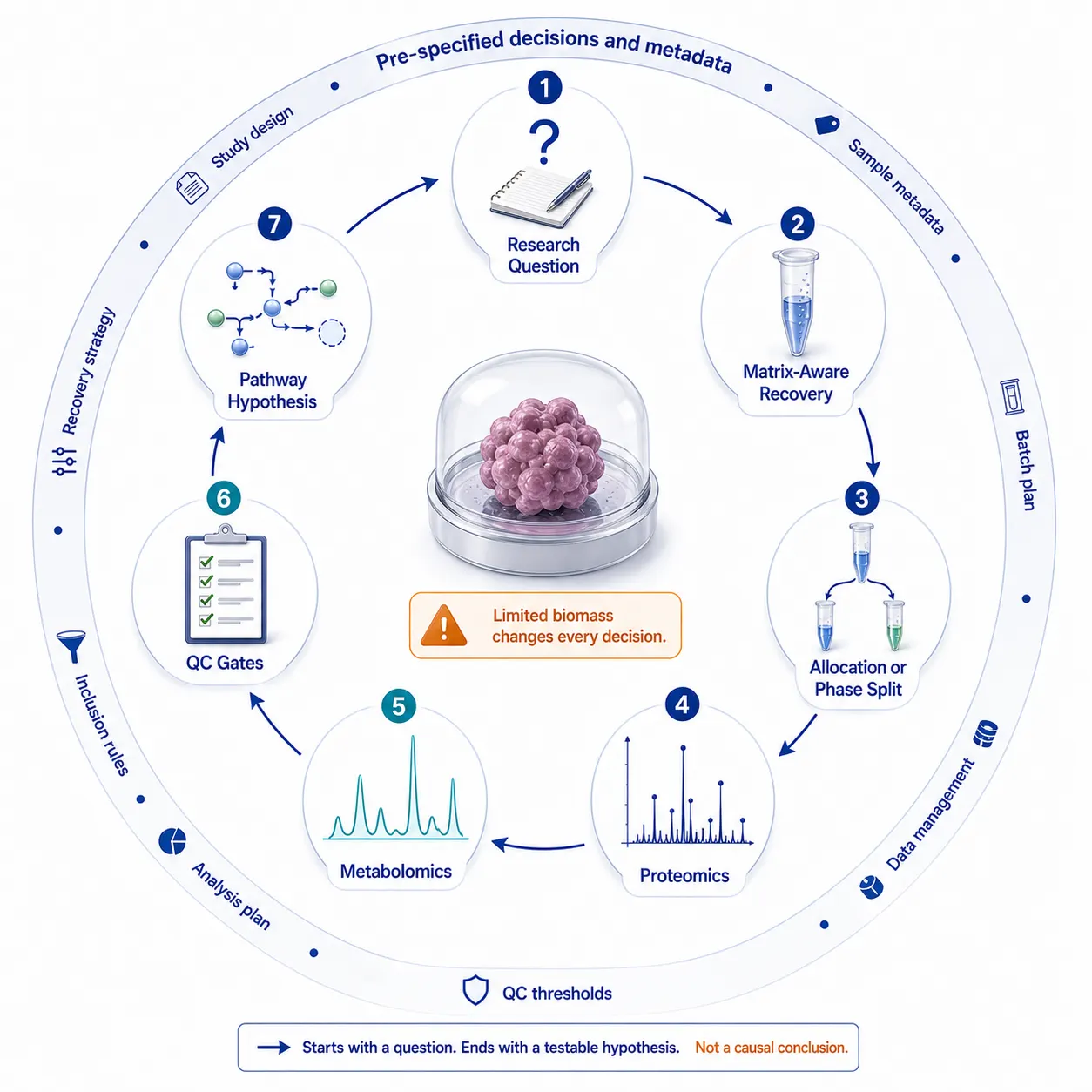 Figure 1. A same-sample organoid multi-omics design begins with the biological question and treats recovery, extraction, and integration as linked evidence decisions.
Why Same-Sample Co-Profiling Is a Design Choice, Not an Automatic Upgrade
Measuring protein and metabolite layers from the same organoid preparation can reduce uncertainty about whether the two assays represent the same perturbation state. This is especially helpful when cultures vary between wells, when the treatment effect is transient, or when the sample is too limited for independent replicate sets. A biphasic extraction can partition polar metabolites, lipids, and a protein-rich interphase from one recovered specimen. The MPLEx workflow is a useful precedent for this architecture: it demonstrates that one sample can support integrative protein, metabolite, and lipid measurements when phase handling and downstream preparation are planned as a system rather than as isolated assays.1
That benefit has limits. The protein interphase is not automatically equivalent to a protein preparation optimized only for deep proteome coverage, and a solvent system that is convenient for broad metabolite coverage may not be ideal for every protein readout. Sample sharing also couples failure modes: incomplete matrix removal, an extraction delay, or a poor phase split affects more than one data layer. For this reason, same-sample analysis is best used when specimen-level correspondence changes the strength of the eventual inference, not merely because it sounds more comprehensive.
Start by assigning every proposed layer a role. One layer may identify a perturbed pathway, another may establish whether a protein family changes consistently with that pathway, and a focused assay may later confirm a small panel. If a layer has no decision it could change, it is a candidate for removal. This simple filter prevents method stacking: the accumulation of attractive technologies that creates more tables but not more interpretable evidence.
Start With Matrix-Aware Sample Recovery
For organoid cultures, recovery is an analytical variable. Basement membrane extract or another hydrogel can contribute proteins, lipids, and small molecules that are not produced by the organoid. It can also suppress or distort measurements indirectly by changing the composition and handling of the recovered material. A clean-looking pellet is not proof that the matrix contribution is negligible. The recovery plan should define what is being removed, what will serve as an extraction blank, and how residual matrix risk will be documented.
Use a recovery approach compatible with the biological model and chosen analytes. Cold, matrix-compatible washes may help reduce carryover, but the specific wash chemistry, handling time, and mechanical force should be optimized and documented rather than copied as a universal recipe. Prepare at least two control types when feasible: a processed matrix-only control that follows the recovery procedure, and a procedural blank that follows the solvent and consumable path. Their role is different. A matrix control helps identify hydrogel-derived features; a procedural blank helps reveal contaminants introduced after recovery.
Because low biomass magnifies handling variation, record the information needed to reconstruct the sample history: model identity, passage or maturation state, culture format, matrix lot, treatment, collection order, operator, recovery method, storage condition, and deviations. A properly designed protein sample preparation service can be useful when recovery, cleanup, and digestion must be tuned around scarce or matrix-rich material. The important deliverable is not simply a clean digest; it is a preparation record that lets the research team distinguish a biological difference from a recovery difference.
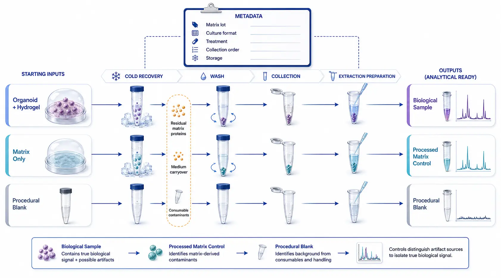 Figure 2. Matrix-aware recovery requires evidence controls, not only a wash step: processed matrix controls, procedural blanks, and sample-history metadata reveal different sources of unwanted signal.
Choose Parallel Allocation or Single-Sample Phase Partitioning Before You Culture
The first fork is whether the two omics layers need to originate from the same recovered specimen. There are two defensible architectures. In parallel allocation, matched organoid cultures are collected into separate proteomics and metabolomics workflows. This allows each workflow to use its preferred lysis, cleanup, and loading strategy. It is often the better choice when the primary endpoint needs maximal depth in one layer, when different workflows require incompatible preservation conditions, or when enough biological replicates can be maintained in both branches.
In single-sample phase partitioning, one recovered specimen is extracted into chemically distinct fractions. This design prioritizes within-sample pairing. It is attractive when the sample is limited, when response heterogeneity between wells is a major concern, or when the central question is whether changes in protein machinery and small-molecule state co-occur in the same specimen. The trade-off is that the extraction cannot be optimized independently for every fraction. A small pilot should therefore test recovery, feature count, precision, and missingness for each layer before the main experiment is committed.
There is also a middle path. Researchers may pool technical material within a biological replicate, then allocate a defined fraction to targeted metabolite confirmation and retain the remainder for proteomics. This is not less rigorous than phase partitioning if the allocation is set before results are seen and the experiment still retains true biological replication. Avoid a universal percentage split. The usable allocation depends on model size, expected abundance range, instrument sensitivity, and the question that matters most if material becomes limiting.
For broad chemical discovery, use an untargeted metabolomics service when the aim is to identify patterns and candidate pathway changes rather than to quantify a short, predefined panel. If the study instead has a small set of decision-critical metabolites, a targeted metabolomics service can provide the focused confirmation step. These are different evidence roles; treating targeted analysis as an afterthought often leaves the project with plausible but unverified features.
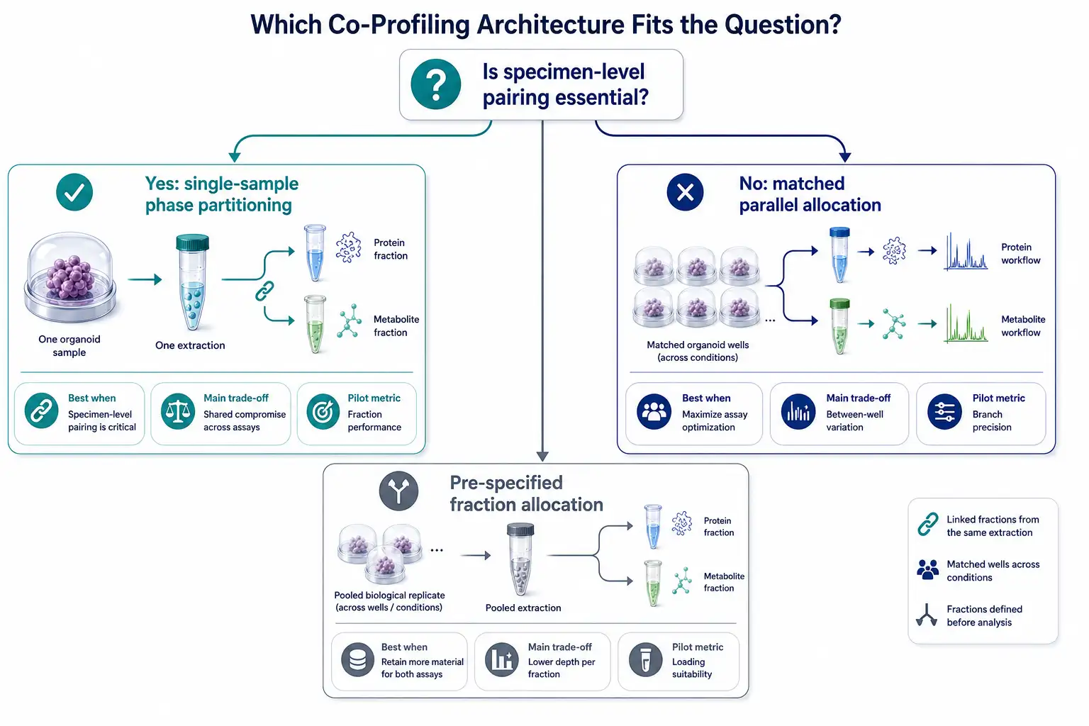 Figure 3. Select same-sample phase partitioning when specimen-level pairing is essential; select parallel allocation when layer-specific optimization or depth is more important.
Build the Extraction Around the Question and the Phase You Need to Keep
A biphasic workflow is a chain of separations. A polar fraction can support many water-soluble metabolites; an organic fraction can support lipid-rich chemistry; and the interphase or pellet can be processed for protein measurement. The operational details should be piloted in the actual organoid matrix, because phase behavior and recoveries are affected by biomass, residual medium, hydrogel carryover, and sample-to-solvent ratio. Do not infer successful co-extraction only from the presence of features. Assess whether those features are reproducible, distinguishable from controls, and fit for the biological comparison.
Design the sequence with the most fragile measurement in mind. If the question centers on labile metabolites, prioritize rapid, consistent quenching and cold handling, then assess whether the resulting protein fraction still meets the planned protein endpoint. If the question centers on proteome depth or low-abundance pathways, it may be more defensible to use dedicated protein preparation and a parallel metabolite branch. For protein quantification, an DIA quantitative proteomics service can be considered when consistent proteome-wide comparison across a planned cohort is the priority, but its feasibility should be evaluated with the actual material rather than assumed from a general tissue workflow.
Write down the fraction-to-analysis map before collection. It should state which fraction goes to discovery analysis, which aliquot is retained for re-analysis, whether a pooled QC is assembled, and what happens if the available material falls below a predefined threshold. The final decision rule matters more than an apparently elegant extraction diagram. A project that defines its fallback route in advance is less likely to make post hoc choices that favor a preferred result.
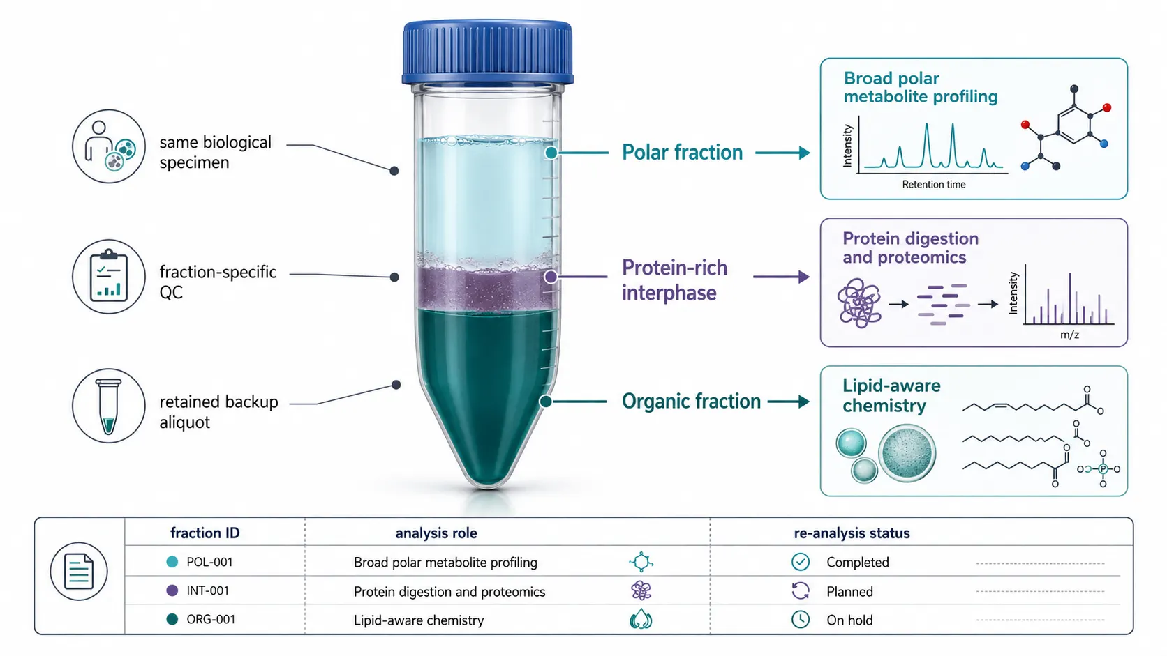 Figure 4. A same-sample biphasic workflow creates linked but non-identical evidence layers; each fraction requires its own recovery, QC, and interpretation criteria.
Normalize Without Mechanically Erasing Biology
Normalization is where multi-omics projects can accidentally turn a real biological shift into an apparently tidy dataset. Organoid models may differ in cell number, differentiation state, extracellular material, viability, and biomass after a perturbation. A single denominator cannot correct every layer without assumptions. Protein amount, DNA, cell count, organoid number, imaging-derived volume, or a spike-in reference may each be informative in a particular design, but none should be treated as a universal gold standard.
Instead, create a biomass and loading ledger. Record the planned biological unit, the amount loaded into each analytical layer, the value used for within-layer normalization, and the reason that reference is appropriate for the analyte class. For example, protein loading may be a practical reference for a proteomics digest; an internal-standard strategy and a feature-specific approach may be more appropriate for metabolite data. If the perturbation itself changes biomass, report that fact as part of the result rather than automatically normalizing it away.
A protein quantification service can support a pre-specified protein loading check, but it should not be used to impose an unexamined biological correction on metabolites. Review how key conclusions behave under reasonable, pre-declared alternatives. If a pathway finding appears only under one aggressive normalization choice, label it as conditional rather than presenting it as a stable cross-omics result.
Build a QC Architecture for Low-Biomass Multi-Omics
Low-input designs need more QC structure, not more confidence language. QC should begin with sample acceptance and continue through extraction, acquisition, and data processing. At minimum, pre-specify sample identifiers, a collection randomization plan, batch order, pooled QC composition, blank positions, internal standards where appropriate, reinjection rules, and the criteria for flagging a sample rather than silently excluding it.
Use pooled QC material to monitor analytical stability, but do not allow it to substitute for biological replication. Pooled QC can reveal drift, retention-time movement, or inconsistent feature response; it cannot estimate the variability between independent organoid cultures. Processed matrix-only controls and procedural blanks help identify features that should be removed or interpreted cautiously. For the proteome layer, review identification completeness, digestion or recovery consistency, and missing-value patterns separately from metabolite feature stability. For metabolite data, review blank contribution, internal-standard behavior, peak-shape suitability, and pooled-QC reproducibility in the context of the chosen analytical method.
For experiments where both layers must be planned together, an integrated proteomics and metabolomics analysis service can help define a coordinated QC and data-integration plan. The key is to maintain layer-specific pass criteria. A sample can be usable for one layer and not another; forcing every sample into a combined analysis often hides this distinction and creates unreliable correlations.
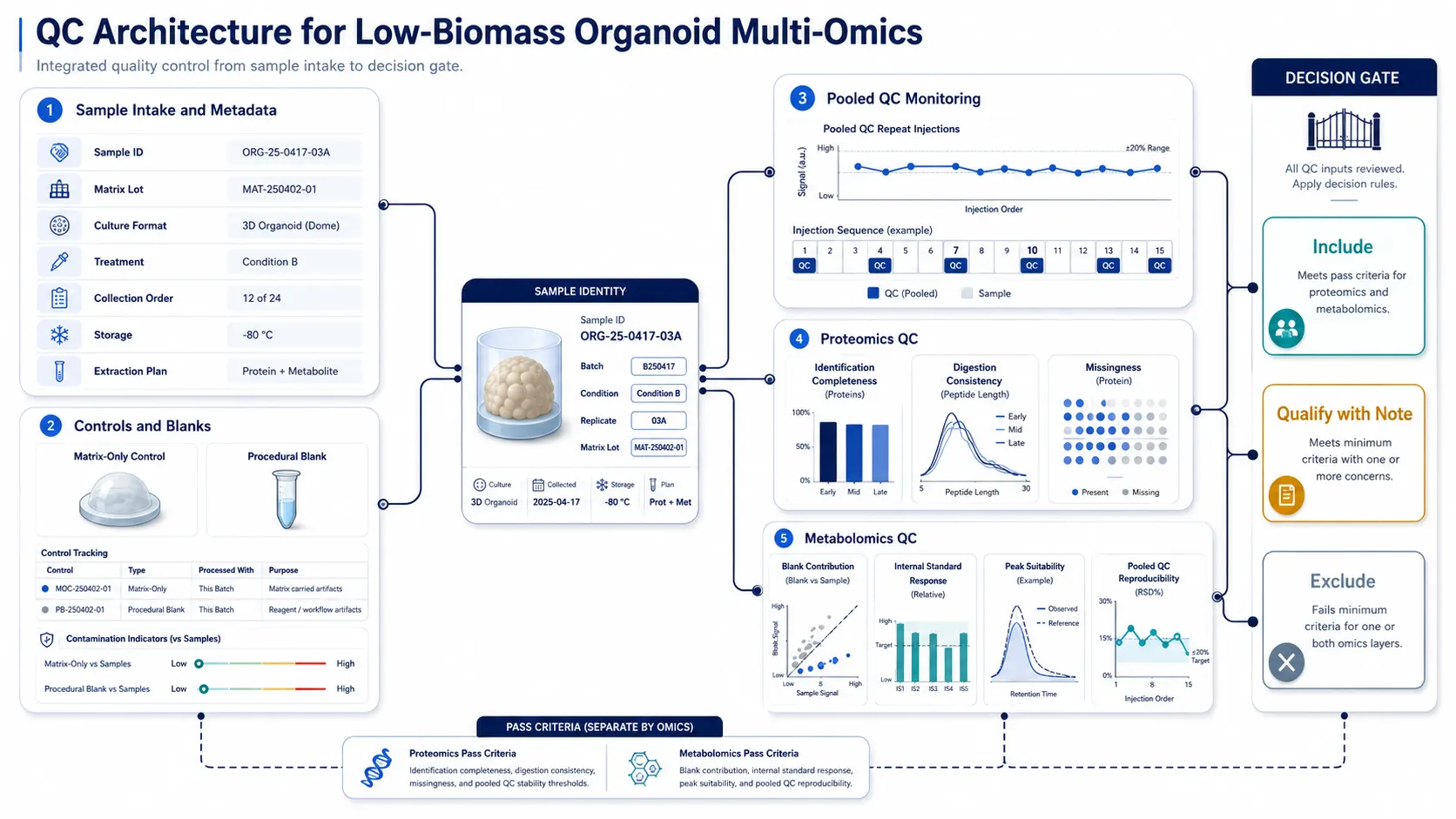 Figure 5. Low-biomass co-profiling needs a layer-specific QC architecture: shared sample tracking, plus separate criteria for proteome and metabolite data quality.
Integrate Pathways Without Turning Correlation Into Causation
Multi-omics integration is most useful when it narrows a biological hypothesis. It is not a license to convert a protein-metabolite correlation into an enzyme-substrate claim. A measured metabolite can reflect transport, medium carryover, extraction behavior, compartmentalization, or multiple reactions; an enzyme abundance change may not represent its activity. Integration should therefore be presented as pathway triangulation: several observations pointing to a candidate process that deserves a follow-up experiment.
Start with a shared annotation layer. Standardize sample identifiers, contrast definitions, time points, species or model identifiers, gene/protein identifiers, metabolite confidence levels, and versions of the pathway resource. Then ask focused questions: Do the altered proteins map to an enzymatic or transport process that is consistent with the direction of a metabolite change? Is the pattern replicated across biological samples? Does it persist after blank filtering and the planned normalization sensitivity check? What additional assay would discriminate competing explanations?
A bioinformatics for proteomics service can support identifier harmonization, enrichment analysis, and traceable reporting, but the experimental team must retain the causal boundary. A useful final figure might show the evidence chain from metabolite feature, to protein family, to pathway, to a proposed validation assay. It should not draw an arrow that implies direct regulation unless an appropriate experiment has tested that relationship.
If phosphorylation is part of the next mechanistic step, the companion guide on paired phosphoproteomics and total-proteome experiments explains how to avoid mistaking abundance changes for site-level regulation. If the follow-up question is whether an unanticipated modification should be discovered broadly or confirmed directly, see open modification search versus targeted PTM analysis. These links extend the evidence chain without making the present experiment responsible for every omics layer.
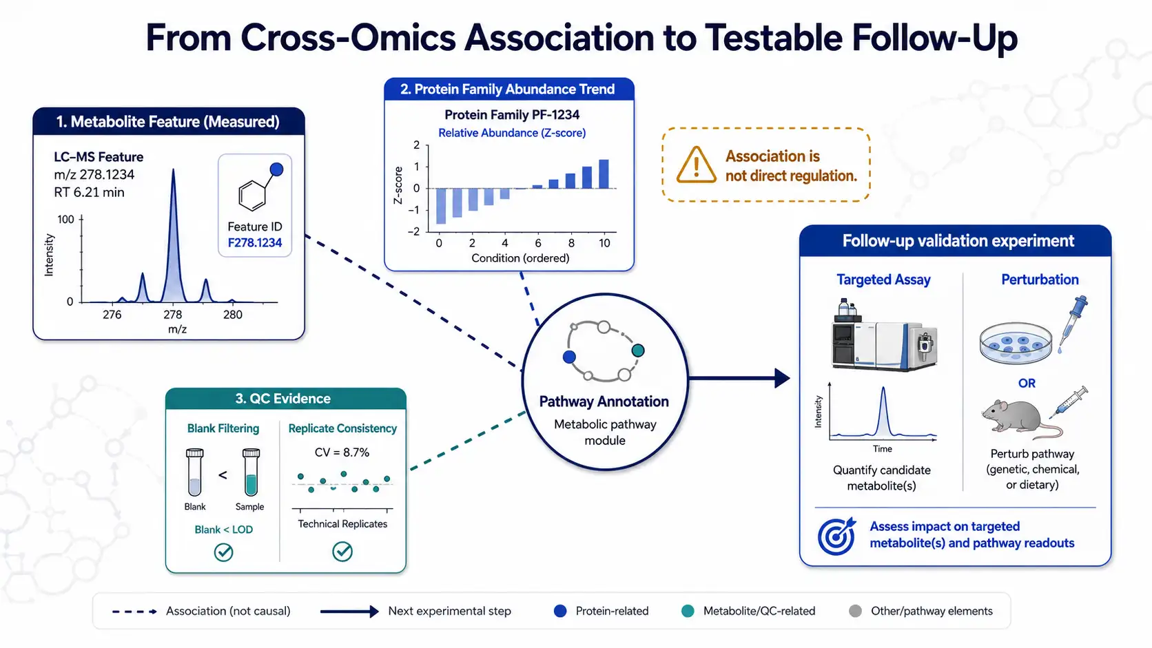 Figure 6. Cross-omics integration should generate testable pathway hypotheses, with associations clearly separated from demonstrated causal mechanisms.
Use a Four-Phase Implementation Plan
Phase 1: define the decision. Write one sentence that states the biological contrast, the organoid model, the unit of replication, and the decision the data must support. Assign a specific role to proteomics, metabolomics, and any focused validation assay. Remove layers that cannot change the decision.
Phase 2: run a small matrix and extraction pilot. Compare the intended recovery method with matrix-only and procedural controls. Test the chosen allocation or phase-partition architecture using representative material. Review feature quality, protein recovery suitability, and missingness before scaling the study.
Phase 3: lock the sample and QC ledger. Predefine identifiers, randomization, handling records, extraction batches, pooled QC, blank placement, acceptance thresholds, and the conditions that trigger re-analysis. Confirm that biological replicates remain biological replicates after any pooling decision.
Phase 4: integrate and challenge the result. Analyze each layer with its own QC logic, harmonize the metadata, and combine only measurements that have passed their relevant checks. For each integrated pathway, state a plausible alternative explanation and name the experiment that could challenge it. This final step turns a broad co-profiling experiment into a credible hypothesis-generating study.
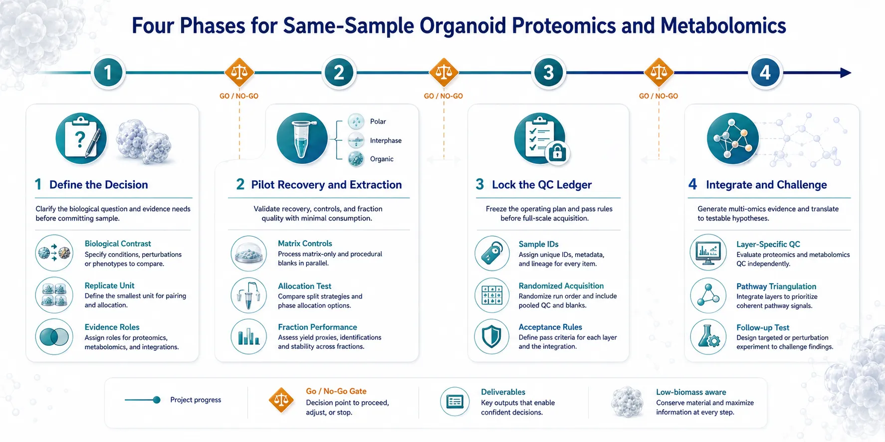 Figure 7. A four-phase implementation plan keeps the study focused on evidence quality: define the decision, pilot the recovery architecture, lock QC, then integrate and challenge the findings.
Recognize the Failure Patterns Before They Reach Integration
Failure pattern 1: the apparent pathway is carried by controls. A visually persuasive metabolite pattern can originate from matrix, medium, plasticware, or a feature that behaves differently across batches. This is why blank subtraction alone is not enough. A feature removed by a procedural blank and a feature associated with a processed matrix-only control are different analytical problems. Keep the control evidence attached to the feature review rather than treating controls as a single pass or fail checkpoint at the beginning of the workflow.
Failure pattern 2: the co-profiling design has no true biological replication. Dividing one pooled specimen into many analytical fractions can improve technical coverage, but it cannot replace independent organoid cultures. If pooling is necessary to obtain enough material, document the pool composition and interpret it as one biological replicate. The remaining design must still contain enough independent biological units to evaluate whether the observed direction is stable. Technical injections, repeat digests, and repeated instrument runs can characterize precision; they do not estimate biological heterogeneity.
Failure pattern 3: a low-input sample is treated like a conventional bulk sample. In limited material, missingness and variability can increase unevenly across fractions. A conclusion should not be built from an apparent decrease when the relevant signal is absent in most replicates or sits near the blank level. Set feature-level review rules before looking at the treatment contrast. Examples include minimum detection completeness, blank-to-sample separation, pooled-QC stability, and a stated approach for values that are not observed. The exact thresholds should fit the method and pilot data, but the governance should be fixed before interpretation.
Failure pattern 4: integration begins after identifiers have drifted. Protein groups, metabolites, samples, and contrast labels often change during separate analysis tracks. A late-stage spreadsheet merge can silently pair the wrong time point, normalize against inconsistent sample labels, or discard confidence information. Maintain one master sample map and one immutable analysis manifest from collection through reporting. Every cross-layer plot should be traceable back to the sample identifier, analytical batch, data-processing version, and feature-confidence rule that produced it.
Failure pattern 5: the study becomes broader after data review. Exploratory analysis is valuable, but it should be labeled as exploratory. Separate pre-specified questions, pilot-derived feasibility findings, and post hoc observations in the final report. That separation is especially important in multi-omics, where a large search space can produce attractive associations by chance. The credibility of the work comes from showing what was planned, what changed, and what needs a targeted follow-up.
Frequently Asked Questions
Is a same-sample workflow always better than matched parallel wells?
No. Same-sample workflows are most valuable when specimen-level pairing is central to the research question or sample scarcity makes parallel branches impractical. Matched parallel wells are often preferable when one layer needs an assay-specific extraction or maximum depth.
Can one extraction protocol preserve every metabolite and every protein measurement?
No universal protocol can optimize all chemical classes and protein endpoints simultaneously. Select the workflow around the key decision, then verify performance in a representative pilot with the actual matrix and planned readouts.
Should protein amount be used to normalize all metabolite results?
Not automatically. Protein amount can be a useful loading or biomass reference in a defined design, but it can also remove a biological change if the perturbation affects biomass. Pre-specify the reference and assess whether key findings are robust to reasonable alternatives.
What controls are most important for hydrogel-grown organoids?
At minimum, consider a processed matrix-only control and a procedural blank, alongside biological samples and pooled QC material. Each addresses a different source of non-biological signal.
Does a protein-metabolite correlation demonstrate pathway activity?
No. It can support a pathway hypothesis, but direct activity, flux, transport, and compartmentalization usually require additional evidence. Report the correlation as an association and design a follow-up assay to test the proposed mechanism.
When should targeted metabolomics be included?
Include it when a small set of metabolites is decision-critical or when discovery features require focused confirmation. Plan the targeted branch before the study starts so retained material, standards, and QC expectations are realistic.
References:
- Nakayasu ES, et al. MPLEx: a Robust and Universal Protocol for Single-Sample Integrative Proteomic, Metabolomic, and Lipidomic Analyses. mSystems. 2016;1(3):e00043-16. https://pmc.ncbi.nlm.nih.gov/articles/PMC5069757/ (CC BY 4.0).
- Gillespie J, et al. Metabolism of parathyroid organoids. Frontiers in Endocrinology. 2023;14:1223312. https://doi.org/10.3389/fendo.2023.1223312 (CC BY 4.0).
- Lindeboom RGH, et al. Integrative multi-omics analysis of intestinal organoid differentiation. Molecular Systems Biology. 2018;14:e8227. https://doi.org/10.15252/msb.20188227 (CC BY 4.0).