Meta Intent: This article addresses a specific pain point for researchers whose spatial proteomics data is already acquired but stalled at the analysis stage — particularly cell type annotation. It explains why tools designed for single-cell/spatial transcriptomics fail when applied directly to protein-level data, and provides a practical framework for performing annotation correctly.
Why Is Cell Type Annotation Harder in Spatial Proteomics Than in Transcriptomics?
At first glance, cell type annotation in spatial proteomics sounds like a solved problem. Single-cell transcriptomics has produced dozens of mature annotation tools — Seurat label transfer, SingleR, CellTypist, scArches — and spatial transcriptomics platforms like Visium and MERFISH routinely use these pipelines. It is tempting to take the same workflow and apply it to your spatial proteomics data.
The problem: it usually does not work well.
Three fundamental differences separate proteomics from transcriptomics when it comes to cell typing:
First, the feature space is much smaller. A typical scRNA-seq experiment measures 3,000–5,000 genes per cell. A spatial proteomics panel — whether on IMC, CODEX/PhenoCycler, MIBI, or DSP — typically measures 20–60 protein markers. Many annotation algorithms rely on high-dimensional nearest-neighbor graphs. With only 40 dimensions instead of 3,000, those graphs become sparse and unreliable.
Second, the data distributions are different. Transcriptomics data follows a negative binomial distribution with frequent zero counts (dropout events). Proteomics data — especially metal-tagged antibody signals on IMC/MIBI — produces continuous intensity values with a different noise structure. Tools that assume transcriptomics-specific distributions will misfire.
Third, mRNA abundance and protein abundance are not the same thing. The correlation between transcript and protein levels is surprisingly modest — typically in the range of R = 0.4–0.6 across studies. A cell type defined by a transcriptomic signature may express those same markers at very different levels at the protein level, or not at all. This means transcriptomics-derived reference atlases do not simply "transfer" to proteomics data.
These differences are not edge cases. They produce systematic misannotation that can propagate through an entire analysis pipeline.
With spatial proteomics panels expanding toward 100-plex and multi-tissue reference atlases proliferating, getting cell type annotation right has moved from a niche concern to a core bottleneck in 2026.
Know Your Data: Spatial Proteomics Platforms and Their Annotation-Relevant Characteristics
Before choosing an annotation strategy, you need to understand what your platform actually measures. Different spatial proteomics technologies produce fundamentally different data structures, and this directly affects which annotation methods are viable.
Imaging Mass Cytometry (IMC) uses metal-conjugated antibodies detected by laser ablation and mass cytometry. A typical IMC experiment measures 35–50 markers at 1 μm resolution. The data output is a multi-channel TIFF stack — essentially an image where each pixel is a mass spectrum. IMC data is continuous-valued, relatively low background, and the main challenge for annotation is that you are working with pixel-level data before segmentation.
Services supporting IMC data analysis are available at Creative Proteomics, including MS-based spatial proteomics service for end-to-end workflows and bioinformatics for proteomics for custom computational pipelines.
CODEX / PhenoCycler uses DNA-barcoded antibodies with cyclic imaging. It typically measures 40–60 markers at subcellular resolution (~0.25 μm). The data is fluorescence-intensity-based with autofluorescence background that requires careful correction. Unlike IMC, CODEX produces optical images that can be directly inspected — this is an advantage for manual validation of annotation results.
MIBI (Multiplexed Ion Beam Imaging) uses metal-conjugated antibodies with secondary ion mass spectrometry, achieving ~0.26 μm resolution with 40–50 markers. MIBI data is similar to IMC in structure but generally has better signal-to-noise ratio due to the ionization method. The higher sensitivity means low-abundance markers (e.g., transcription factors, phosphorylated proteins) are more reliably detected.
GeoMx DSP (Digital Spatial Profiling) is fundamentally different: it measures protein expression from user-selected regions of interest (ROIs), not at single-cell resolution by default. A typical experiment profiles 60–80 proteins across dozens of ROIs. Cell type annotation on DSP data requires a different approach — you are annotating regions, not individual cells, and the analysis logic is closer to bulk proteomics deconvolution than to single-cell annotation.
MALDI-MSI (Matrix-Assisted Laser Desorption/Ionization Mass Spectrometry Imaging) measures hundreds of endogenous peptides and proteins directly from tissue sections without antibody labeling. The data is spectral — each pixel contains a mass spectrum — and annotation workflows must handle the added complexity of peptide identification before cell typing can even begin.
For labs working with FFPE tissues, Creative Proteomics offers FFPE spatial proteomics service optimized for archival tissue specimens.
Each platform produces data that looks different to an annotation algorithm. A method that works beautifully on 50-marker IMC data may fail completely on 80-plex DSP ROI data. Platform-aware workflow selection is the first step toward reliable annotation.
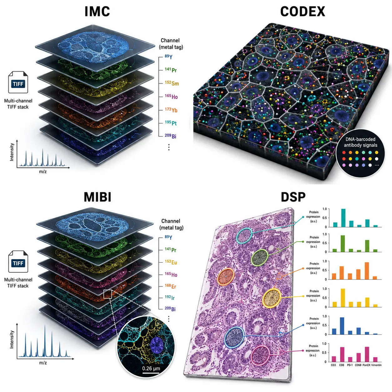 Figure 1. Comparison of data structures across four major spatial proteomics platforms — IMC, CODEX, MIBI, and DSP.
Six Ways Transcriptomics Annotation Tools Fail on Proteomics Data
Understanding what goes wrong is more useful than simply knowing that something goes wrong. Here are six specific failure mechanisms, each with a concrete example.
Mechanism 1: Dimensionality Collapse
Transcriptomics tools like Seurat's label transfer operate in PCA space with 30–50 principal components. When your input data only has 40 markers to begin with, PCA further compresses an already sparse feature space. The result: cell clusters that should be distinct (e.g., CD8+ effector memory vs. CD8+ naive T cells) collapse into a single blob because the algorithm cannot "see" the relevant dimensions.
The fix: skip PCA-based dimensionality reduction for proteomics data. Use all available markers directly, or apply supervised feature selection rather than unsupervised compression. If you must reduce dimensionality for visualization, use t-SNE or UMAP on the raw marker space, but perform annotation in the full feature space.
Mechanism 2: Scale Mismatch Between Reference and Query
Label transfer methods (Seurat, Symphony, scArches) work by finding mutual nearest neighbors between a reference dataset and the query. The reference is typically built from scRNA-seq data where each gene is measured on a log-normalized count scale. The query — your proteomics data — has intensity values on an arcsinh or z-score scale. The distance metrics don't line up.
This is not just a normalization issue. It is a distributional mismatch. Even after applying the same transformation to both datasets, the underlying data-generating processes are different (mRNA molecules vs. metal ions hitting a detector).
Mechanism 3: Marker Gene Set Collapse
Annotation tools like CellTypist and SingleR rely on curated marker gene lists — sometimes hundreds of genes per cell type — to score and assign labels. With a 40-plex proteomics panel, you may have only 2–4 of those markers available for a given cell type. The scoring function degrades rapidly as the marker set shrinks.
A T cell annotation that uses CD3D, CD4, CD8A, FOXP3, and 20 other genes in transcriptomics space collapses to CD3, CD4, and CD8 in proteomics space. The algorithm can distinguish CD4+ from CD8+ T cells but loses the resolution to separate regulatory T cells from conventional CD4+ T cells.
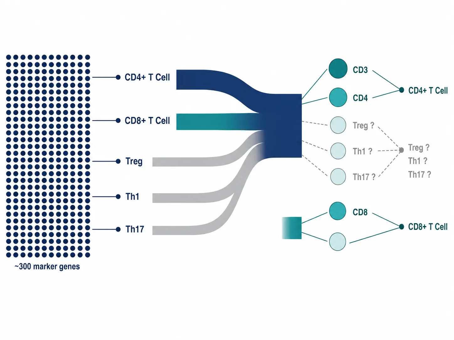 Figure 2. Marker gene set collapse — transcriptomics panel with 300+ marker genes per cell type vs. proteomics panel with 2–5 protein markers.
Mechanism 4: Zero-Inflated Model Assumptions
Many single-cell analysis tools model gene expression as a zero-inflated negative binomial (ZINB) distribution — explicitly accounting for the fact that many genes show zero counts due to dropout. Proteomics data from IMC, MIBI, and CODEX does not have dropout in the same sense. A zero in proteomics data means the protein is genuinely absent (or below the limit of detection). Algorithms that apply ZINB-based imputation or normalization to proteomics data introduce artifacts — they "impute" signal where none exists.
Mechanism 5: Spatial Context Is Ignored
Most transcriptomics annotation tools were designed for dissociated single-cell data — cells in suspension, no spatial information. Even tools adapted for spatial transcriptomics often treat spatial coordinates as an afterthought. In spatial proteomics, however, spatial context is often the most informative feature. A cell expressing cytokeratin and E-cadherin surrounded by CD31+ endothelial cells is almost certainly an epithelial cell in a tissue structure. Ignoring spatial context discards half the information in your dataset.
For labs performing integrated multi-omics analysis, Creative Proteomics provides integrated transcriptomic and proteomic analysis services that combine proteomics with transcriptomics data for more robust annotation.
Mechanism 6: Batch Effects Dominate Biological Signal
The proteomics equivalent of batch effects — variation in antibody staining intensity, laser power fluctuation, metal tag sensitivity differences — can be larger than the biological differences between cell types. Transcriptomics tools that use batch correction methods like Harmony or CCA assume batch effects follow certain parametric forms. These assumptions often fail on proteomics data, where the dominant source of technical variation (antibody lot-to-lot variability) behaves differently from the dominant source in transcriptomics (library preparation batch).
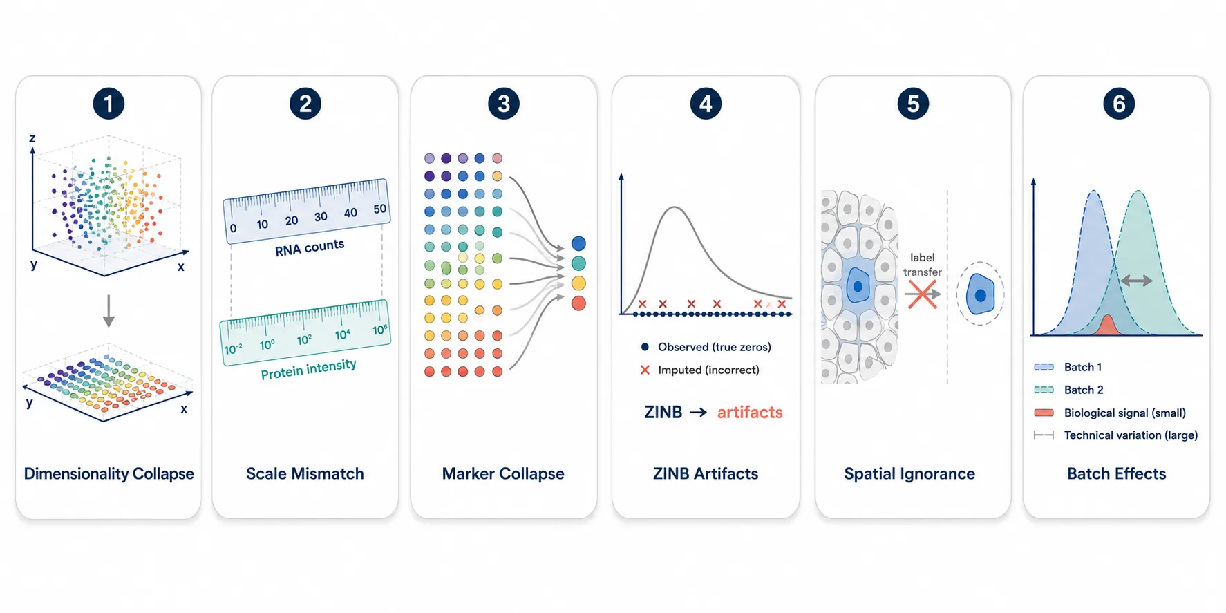 Figure 3. A visual summary of the six failure mechanisms, each illustrated with a simple schematic.
Building a Proteomics-Native Annotation Pipeline: Core Components
Now that we know what breaks, let's build what works. A proteomics-native cell type annotation pipeline has four core components that differ from transcriptomics workflows.
Component 1: Quality Control and Preprocessing
Start with pixel-level or cell-level filtering. For IMC/MIBI data, remove pixels with low total ion count and channels with consistently zero signal across the tissue. For CODEX, apply cyclic normalization to correct for signal decay across imaging cycles. For all platforms, perform channel-wise percentile normalization (e.g., 99.5th percentile) rather than global scaling, which can amplify noise in low-signal channels.
A critical preprocessing step unique to proteomics is metal tag background correction. Metal-conjugated antibodies on IMC and MIBI produce a small but measurable background signal from non-specific binding and incomplete washing. This background varies by tissue type, antibody, and metal tag. Use a Gaussian mixture model per channel to separate true signal from background rather than applying a uniform threshold.
For laser-capture microdissection-based spatial proteomics, Creative Proteomics offers LCM spatial proteomics service with optimized tissue processing protocols.
Component 2: Cell Segmentation
This step has no direct equivalent in single-cell transcriptomics (where cells are already dissociated) and is often the rate-limiting step for annotation quality. Deep learning-based segmentation tools — DeepCell, Cellpose, StarDist — have largely replaced watershed-based methods for IMC and MIBI data, but they require training data or careful fine-tuning for your specific tissue type.
Poor segmentation creates "mixed" cells that express markers from two adjacent cell types, confusing any downstream annotation algorithm. Spend time here. A good segmentation mask is worth more than a sophisticated annotation algorithm.
Component 3: Feature Engineering for Proteomics
Instead of relying on the raw marker intensity matrix, engineer features that amplify biological signal:
- Marker ratios: CD4/CD8 ratio, CK/Vimentin ratio (epithelial vs. mesenchymal)
- Co-expression scores: number of immune markers co-expressed per cell
- Spatial features: distance to nearest blood vessel (CD31+ cell), neighborhood composition (fraction of neighboring cells that are immune vs. stromal)
- Texture features: local standard deviation of marker intensity (helps identify cells at tissue boundaries)
These engineered features capture biological information that would otherwise require many more markers to represent.
Component 4: Annotation Algorithm Selection
Choose your annotation method based on data characteristics, not based on what is popular in transcriptomics. The next sections detail three practical approaches.
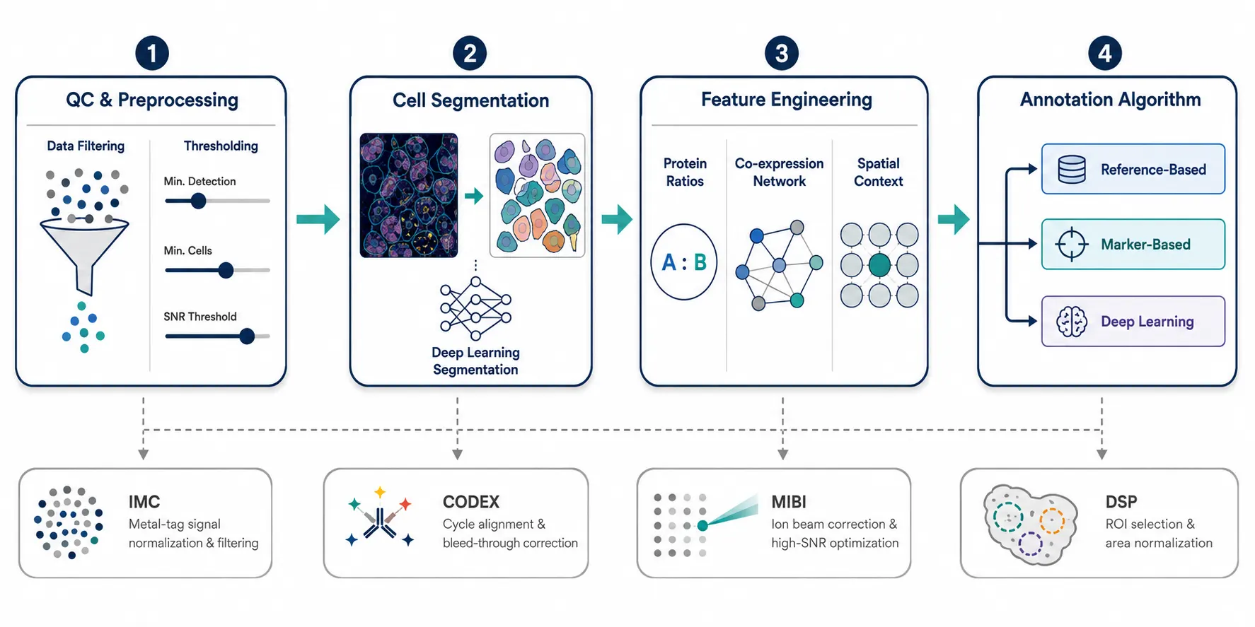 Figure 4. End-to-end pipeline flowchart showing the four core components — QC/Preprocessing to Cell Segmentation to Feature Engineering to Annotation Algorithm Selection.
Annotation Method 1: Reference-Based Label Transfer (with Proteomics-Specific Modifications)
Reference-based annotation maps cell types from a labeled reference dataset to your query data. In proteomics, this approach works — but only with substantial modifications.
Step 1: Build or Obtain a Proteomics Reference
Transcriptomics references (e.g., the Human Cell Atlas, Tabula Sapiens) are not suitable as proteomics references. You need a reference built from proteomics data — ideally from the same or similar tissue, measured on the same or similar platform.
Options for proteomics references:
- TACCO (Transfer of Annotation to Cell types and Conditions): a probability-based label transfer framework that can use proteomics references and handles the smaller feature space natively. It uses optimal transport rather than nearest-neighbor matching, making it more robust to distributional differences.
- STELLAR: designed specifically for spatial proteomics, uses a neural network trained on annotated proteomics data. It learns a mapping from marker combinations to cell types, bypassing the gene-to-protein correlation problem entirely.
- scProAtlas: a spatial proteomics reference atlas covering multiple human tissues, built from IMC and CODEX data. Provides pre-annotated references for common tissue types.
- Build your own: annotate 5,000–10,000 cells manually and train a k-nearest neighbor classifier. This is labor-intensive but often more accurate than using a generic reference that does not match your tissue or panel.
Step 2: Match the Feature Space
The reference and query must use a compatible marker set. If your reference was built with a 50-marker panel and your query uses a different 40-marker panel, find the intersection and work within that shared feature space. If the intersection is too small (<15 markers), reference-based methods become unreliable — switch to marker-based annotation.
Step 3: Apply Distribution Alignment
Before transferring labels, align the intensity distributions between reference and query using quantile normalization or mutual nearest neighbor (MNN) correction. This is analogous to batch correction in transcriptomics but targeted at the specific scale differences in proteomics data.
Step 4: Evaluate Transfer Confidence
Do not blindly trust transferred labels. For each cell, compute a confidence score — the distance to the nearest reference neighbor divided by the distance to the second-nearest neighbor (the "silhouette-like" metric). Cells with low confidence scores (ambiguous mapping) should be flagged for manual review.
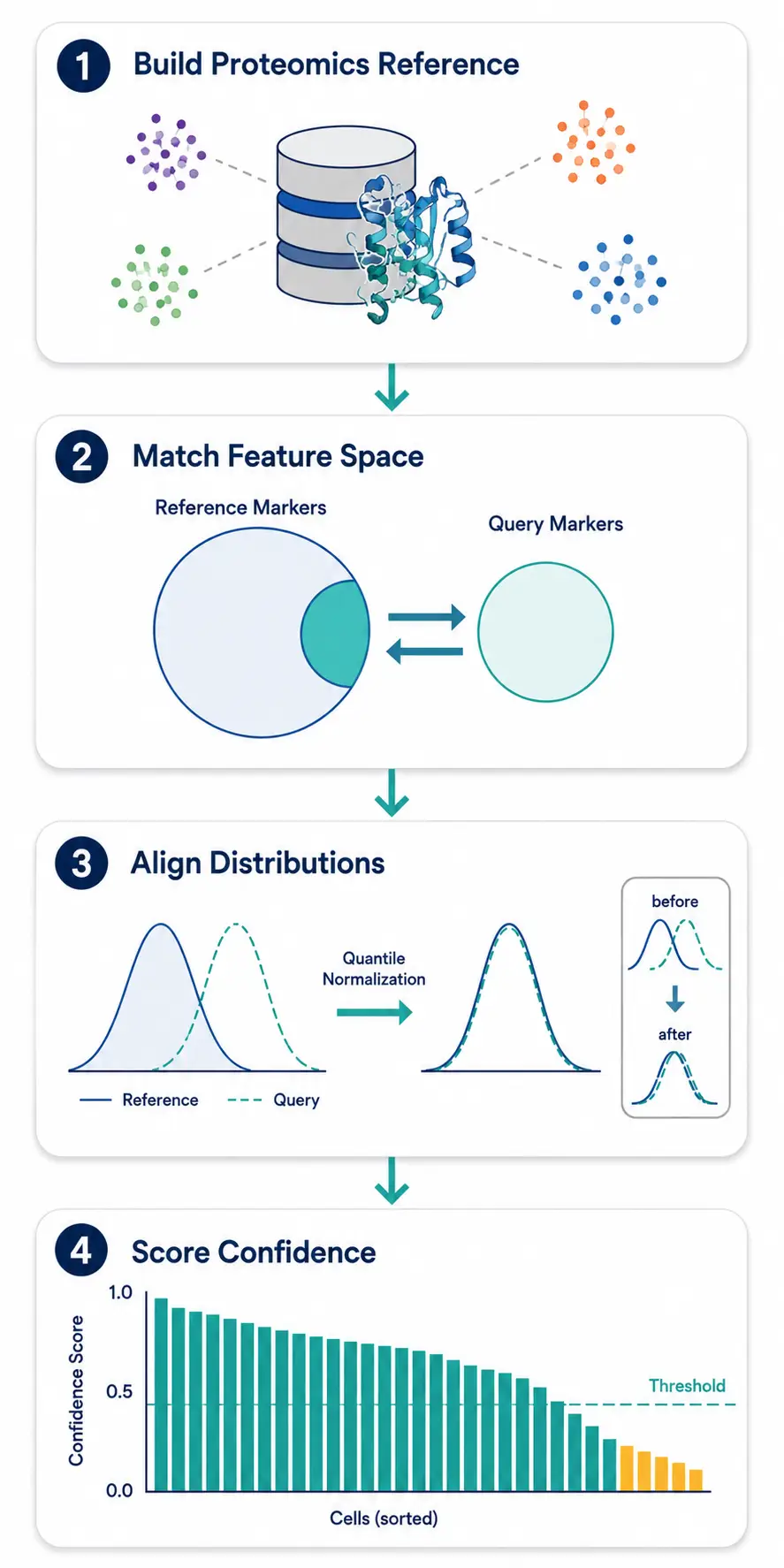 Figure 5. Reference-based label transfer workflow adapted for proteomics — building a proteomics reference to feature space matching to distribution alignment to confidence scoring.
Annotation Method 2: Marker-Based Semi-Supervised Annotation
Marker-based annotation uses known protein markers to define cell types through manually specified rules. This is the most transparent method and often the most accurate for well-characterized tissues — but it requires expert knowledge to define the rules correctly.
Defining Annotation Hierarchies
Build a decision tree rather than a flat list of marker combinations. A practical hierarchy for a tumor microenvironment sample:
Level 1 (Broad lineage):
- Pan-cytokeratin (PanCK) high → Epithelial / Tumor
- CD45 high → Immune
- CD31 high → Endothelial
- α-SMA high, PanCK low, CD45 low → Stromal / Fibroblast
Level 2 (Immune sub-lineage):
- CD3 high → T cell
- CD20 high → B cell
- CD68 high → Myeloid
Level 3 (T cell subtypes):
- CD3+ CD4+ → CD4 T cell
- CD3+ CD8+ → CD8 T cell
- CD3+ CD4+ FOXP3+ → Regulatory T cell
The key advantage of marker-based annotation is that you control the logic. If a cell is CD3+CD8+, you know exactly why it was labeled a CD8 T cell. There is no black box.
Handling Ambiguous Cells
Real data is messy. Cells at tissue boundaries often co-express markers from two lineages (e.g., CD45+PanCK+). Instead of forcing a single label, introduce an "ambiguous" or "double-positive" category. These cells often represent biologically meaningful populations — tumor-immune interactions or epithelial-mesenchymal transition intermediates.
IMmuneCite is a semi-supervised framework designed for spatial proteomics that combines marker-based rules with a probabilistic scoring system. It allows users to define hierarchical marker rules and then assigns each cell a probability vector across all cell types rather than a single hard label.
For marker panel design before starting your experiment, Creative Proteomics provides customized experiment design services with expert-guided panel optimization.
Annotation Method 3: AI/Deep Learning Approaches
Deep learning methods are emerging as powerful annotation tools for spatial proteomics, particularly for datasets where marker-based rules are insufficient and a suitable reference does not exist.
RIBCA (Reference-Image-Based Cell Annotation, 2025)
RIBCA uses histological image features to guide cell type annotation. The key insight: cell morphology in H&E or IMC channel images contains information that protein marker panels miss. A fibroblast and a myofibroblast may have similar marker profiles (both α-SMA+) but look different morphologically. RIBCA trains a convolutional neural network on the image data and uses the learned features as additional "markers" for annotation.
DeepCell Types
An extension of the DeepCell segmentation framework that jointly performs segmentation and cell type classification. It uses a single neural network that takes raw multi-channel images as input and outputs both cell boundaries and cell type labels. The advantage: segmentation and annotation share feature representations, so the model learns that cells of the same type tend to have similar morphology and that tissue architecture informs both tasks.
AnnoSpat (2024)
A graph neural network approach that explicitly models spatial relationships between cells. Each cell is a node in a graph, connected to its spatial neighbors. The GNN learns to propagate and refine cell type assignments based on both marker expression and neighborhood context. AnnoSpat is particularly effective for tissues with strong spatial organization — lymphoid organs, brain tissue, and tumor-stroma interfaces.
When to Use Deep Learning
Deep learning methods work best when:
- You have a large, well-annotated training dataset (thousands of cells)
- The tissue architecture is complex (e.g., tumor microenvironment, brain)
- Marker-based rules fail because cell types in your system are defined by continuous gradients rather than binary marker expression
When to avoid:
- You have a small dataset (<5,000 cells)
- The tissue is simple and well-characterized (e.g., tonsil, lymph node)
- You need explainable results for publication or regulatory submission
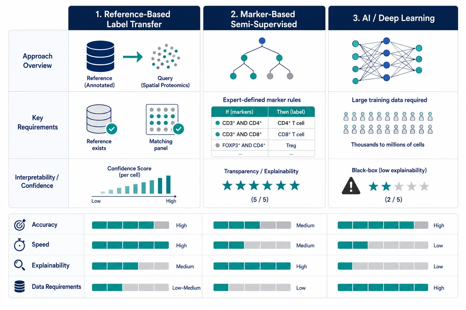 Figure 6. Comparison of the three annotation approaches — reference-based, marker-based, and AI/deep learning — with decision matrix.
Practical Decision Framework: Which Method Should You Use?
The choice of annotation method depends on your specific situation. Here is a practical decision framework.
Start by asking three questions:
- Does a high-quality proteomics reference exist for your tissue and panel?
Yes → Start with reference-based label transfer (Method 1), validate with marker-based checks.
No → Skip to question 2. - Do you have well-characterized protein markers for all expected cell types?
Yes → Use marker-based semi-supervised annotation (Method 2). Build a hierarchical decision tree.
No → Skip to question 3. - Do you have at least 5,000 manually annotated cells for training?
Yes → Consider deep learning (Method 3), especially if tissue architecture is complex.
No → Return to Method 2 with conservative marker rules. Accept that some cells will remain unannotated.
In practice, most projects use a hybrid approach: marker-based rules for major lineages (epithelial, immune, stromal), reference-based transfer for fine subtypes, and manual review for ambiguous cells. This gives you the transparency of rule-based annotation with the coverage of reference-based methods.
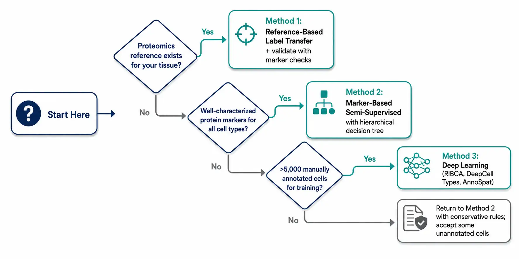 Figure 7. Decision tree flowchart — three branching questions leading to recommended annotation strategies.
Using Spatial Context to Improve Annotation Accuracy
Spatial information is not just a bonus — it is often the decisive factor in resolving ambiguous annotations. Here are concrete ways to use it.
Neighborhood Composition Analysis
For each cell, compute the cell type composition of its local neighborhood (e.g., the 50 nearest cells or all cells within a 20 μm radius). A cell expressing low levels of CD3 in a neighborhood that is 80% CD3+ T cells is probably a T cell with low marker expression. The same cell surrounded by PanCK+ tumor cells might be a tumor cell with non-specific CD3 staining.
Spatial Co-occurrence Priors
Some cell type pairs are biologically expected to co-occur in specific patterns. CD8+ T cells and tumor cells are often adjacent in the tumor microenvironment. CD4+ T cells and B cells cluster together in lymphoid follicles. Build a prior matrix of expected spatial relationships and use it to weight annotation probabilities — a label that respects known tissue architecture is more likely to be correct.
Distance-to-Structure Features
Compute the distance from each cell to key tissue structures. Distance to the nearest CD31+ blood vessel, distance to the tumor-stroma boundary, distance to necrotic regions. These distances are often correlated with cell type: perivascular macrophages are near blood vessels, tumor-infiltrating lymphocytes are inside the tumor region, and fibroblasts are concentrated in the stromal compartment.
AnnoSpat (described above) is the most mature tool for systematic spatial-aware annotation, but even simple spatial features (neighborhood CD45+ fraction, distance to nearest vessel) substantially improve standard marker-based classifiers. Adding spatial features to a random forest classifier trained on marker expression data typically improves annotation accuracy by 5–15 percentage points on held-out test data.
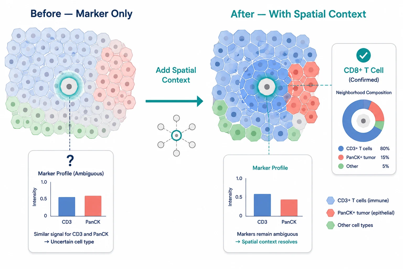 Figure 8. Spatial context correcting annotation — left panel shows ambiguous cell; right panel shows same cell with spatial context providing decisive evidence.
Validation: How to Know Your Annotation Is Correct
Annotation without validation is guesswork. Here is a practical validation framework.
Internal Validation Metrics
- Marker consistency score: For each cell type, compute the mean expression of its defining markers across all cells assigned to that type. Low consistency suggests annotation problems.
- Silhouette score per cell type: Measures how similar cells of the same type are to each other vs. cells of other types. Cell types with low silhouette scores may be poorly defined.
- Neighborhood homogeneity: In well-annotated data, spatial neighbors tend to share cell type labels (tissues are organized). Low neighborhood homogeneity may indicate annotation errors.
External Validation
- Manual expert review: Randomly sample 200–500 annotated cells and have a domain expert assign ground-truth labels. Compare algorithmic labels to expert labels — this gives you a direct accuracy estimate.
- Serial section validation: If you have a serial section stained with conventional IHC or H&E, compare annotation results to what is visible in the serial section. This is especially useful for validating tumor vs. stroma assignments.
- Functional validation: Do the annotated cell types make biological sense? If your annotation says a region is a lymphoid follicle, the cell type composition should be predominantly B cells (CD20+) with scattered CD4+ T cells. If not, the annotation is suspect.
Common Validation Pitfalls
- Circular validation: Do not validate annotation accuracy using the same marker rules you used for annotation.
- Over-reliance on a single metric: All metrics have blind spots. Use multiple complementary metrics.
- Ignoring spatial patterns: An annotation that looks fine at the single-cell level may be nonsensical at the tissue level. Always inspect spatial maps of your annotated cell types.
For complex projects, Creative Proteomics provides statistical analysis services for rigorous spatial statistics and annotation validation, as well as functional annotation services for downstream biological interpretation.
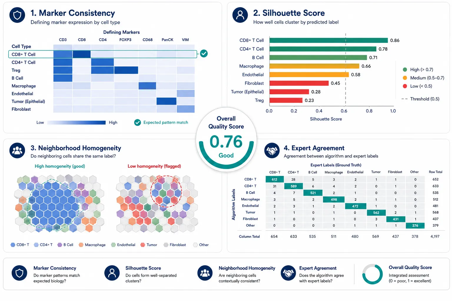 Figure 9. QC and validation framework overview — dashboard-style illustration showing key quality metrics.
When Manual Annotation Is Still the Best Choice
Despite advances in automated annotation, manual annotation remains the gold standard for certain situations. Know when to invest the time.
Situations Where Manual Annotation Is Preferred:
- Novel tissue types or disease states with no existing reference
- Small datasets (<10,000 cells) where automation overhead exceeds manual effort
- Heterogeneous tumors where every sample is biologically unique
- Validation datasets for publication, where ground truth is required
- Datasets with unusual marker combinations that violate algorithm assumptions
How to Do Manual Annotation Efficiently:
- Use interactive visualization tools — napari, QuPath, or ImageJ with the spatial proteomics plugin — to view multi-channel images
- Annotate in hierarchical passes: first broad lineages (epithelial, immune, stromal), then subtypes
- Record the evidence for each annotation decision (which markers, which spatial features)
- Use automated pre-labeling to speed up the process: let an algorithm propose labels, then manually correct errors. Correcting is faster than annotating from scratch
Manual annotation is not a failure of automation. It is a deliberate choice for high-stakes analyses where accuracy matters more than speed. Even in automated pipelines, manual review of a subset of cells is essential for quality control.
Troubleshooting: Common Annotation Problems and Their Solutions
Problem: Two cell types that should be distinct are being merged into one cluster.
Likely cause: Your marker panel lacks distinguishing markers for these subtypes. Check whether any markers that are differentially expressed between these cell types in the literature are missing from your panel.
Solution: If adding markers is not possible, accept the merged annotation and report it as a combined category (e.g., "CD4+ T cells" rather than attempting Th1/Th2/Th17/Treg subtyping).
Problem: A single marker dominates the annotation, suppressing all other signals.
Likely cause: The marker has a very high dynamic range compared to the rest of the panel, and distance-based algorithms overweight it.
Solution: Apply per-channel standardization (z-score) before annotation so all markers contribute equally to distance calculations.
Problem: Annotation results look different between tissue regions despite similar biology.
Likely cause: Spatial variation in antibody penetration or staining efficiency. Deeper tissue regions often show weaker signal.
Solution: Apply regional normalization — normalize each spatially contiguous tissue region independently before annotation.
Problem: CD45+ cells are being annotated as epithelial due to non-specific PanCK signal.
Likely cause: Antibody cross-reactivity or spillover from a highly expressed channel into adjacent mass channels (IMC/MIBI).
Solution: Check the raw spectra — spillover creates a characteristic pattern. Apply compensation matrices (similar to flow cytometry compensation) to correct channel cross-talk before annotation.
How to Choose a Spatial Proteomics Service Provider for Cell Type Annotation
If you are outsourcing your spatial proteomics analysis, four criteria separate a specialist who understands the proteomics-specific challenges covered in this article from a generalist CRO.
Panel Design: Proteomics-Aware Marker Selection
The annotation you can perform is entirely determined by the panel you designed before data acquisition. A specialist provider helps you select markers that resolve your specific cell types at the protein level — accounting for the fact that mRNA-based marker lists often miss key proteomic distinctions, as discussed in the failure mechanisms above. Creative Proteomics provides customized experiment design services with expert-guided marker selection that accounts for protein-level expression patterns, antibody clone performance, and metal-tag compatibility across IMC, CODEX, MIBI, and DSP platforms.
Pipeline Transparency: Know How Your Annotation Was Produced
A specialist provider explains exactly which algorithms and reference datasets were used — whether reference-based label transfer (Method 1), marker-based rules (Method 2), or deep learning (Method 3) as described earlier. If you cannot get a clear explanation of the annotation logic, the output is a black box — and black boxes are risky for publication. Creative Proteomics provides MS-based spatial proteomics services covering the full analysis workflow from raw spatial proteomics data through annotated cell type maps, with each annotation decision traceable to its underlying algorithm or marker rule.
Validation That Matches Publication Standards
Look for a provider that delivers per-cell annotation confidence scores, marker expression heatmaps by cell type, and spatial maps showing that annotated cell types respect tissue architecture — exactly the QC framework described in the Validation section above. A provider should also explain how they handle ambiguous cells and what thresholds they use, rather than silently forcing every cell into a category. Creative Proteomics supports this with dedicated statistical analysis services for rigorous spatial statistics and functional annotation services for downstream biological interpretation.
Customization for Your Biological Question
Your biological question is unique. A specialist provider tailors their annotation pipeline to your needs — building a custom marker hierarchy for a rare cell population, training a bespoke deep learning model on your tissue type, or performing manual annotation of critical cell subsets. For projects requiring fully bespoke experimental and computational design, customized experiments service is available to build end-to-end solutions that match your specific research context, not a one-size-fits-all template.
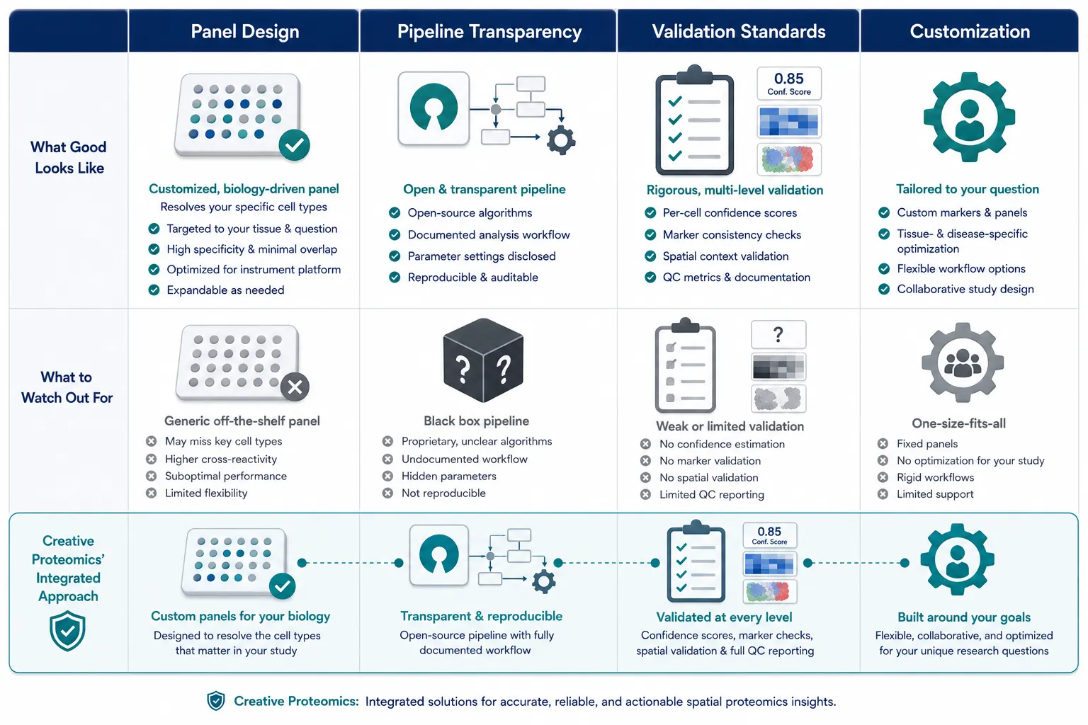 Figure 10. Comparison table summarizing key criteria for evaluating spatial proteomics service providers.
FAQ
Q: Can I use Seurat's label transfer on my IMC data?
A: You can technically run it, but the results will be unreliable because Seurat expects transcriptomics-scale feature spaces and RNA-specific distributions. If you must use Seurat, limit it to proposing candidate labels for manual review rather than accepting its output as final.
Q: What is the minimum number of protein markers needed for reliable cell type annotation?
A: For major lineages (epithelial, immune, endothelial, stromal), 15–20 well-chosen markers are sufficient. For immune subtyping (e.g., separating T cell subsets), you will need 30–40 markers. Below 15 markers, restrict annotation to broad categories.
Q: How long does annotation take for a typical spatial proteomics dataset?
A: Automated annotation of a 1 cm² tissue section with 100,000 cells takes minutes to hours computationally. Manual annotation of the same dataset takes days to weeks. Most projects spend 80% of their time on validation and refinement, not on the initial annotation run.
Q: My GeoMx DSP data is ROI-level, not single-cell. Can I still do cell type annotation?
A: Yes, but the approach is different. DSP ROI annotation is essentially a deconvolution problem — you are estimating the cell type composition within each ROI based on the aggregate protein expression. Tools like SpatialDecon and CIBERSORTx (adapted for proteomics) are more appropriate than single-cell annotation tools.
Q: Can I combine transcriptomics and proteomics data for better annotation?
A: Yes, and this is one of the most active areas of development. Integrated spatial multi-omics (e.g., spatial CITE-seq, or paired Visium + IMC on serial sections) can use transcriptomics for cell type discovery and proteomics for spatial localization. The practical challenge is data alignment across modalities.
Q: What are the key quality metrics reviewers look for in spatial proteomics annotation?
A: Reviewers typically expect: (1) a clear description of the annotation method and rationale, (2) validation against an independent method (manual review or serial section IHC), (3) per-cell confidence metrics, and (4) spatial maps showing that annotated cell types respect tissue architecture.
References
- Mi Z, Yao Y, Li Z, et al. (2024). "Computational methods and biomarker discovery strategies for spatial proteomics: a review in immuno-oncology." Briefings in Bioinformatics, 25(5), bbae421. DOI: 10.1093/bib/bbae421. Open Access.
- Faryabi A, Fasolino M, Patil A, et al. (2024). "AnnoSpat annotates cell types and quantifies cellular arrangements from spatial proteomics." Nature Communications, 15, 3744. DOI: 10.1038/s41467-024-47334-0. CC BY 4.0.
- Magness A, Colliver E, Enfield K, et al. (2024). "Deep cell phenotyping and spatial analysis of multiplexed imaging with TRACERx-PHLEX." Nature Communications, 15, 48870. DOI: 10.1038/s41467-024-48870-5. CC BY 4.0.
- Shaban M, Bai Y, Qiu H, et al. (2024). "MAPS: pathologist-level cell type annotation from tissue images through machine learning." Nature Communications, 15, 438. DOI: 10.1038/s41467-023-44188-w. CC BY 4.0.
- Sun H, Yu Q, Martinez Casals G, et al. (2025). "RIBCA: Robust image-based cell annotation for multiplexed tissue imaging." Cell Systems, 16(9), 101374. DOI: 10.1016/j.cels.2025.101374. CC BY.
- Marconato L, Palla G, Yamauchi KA, et al. (2025). "SpatialData: an open and universal data framework for spatial omics." Nature Methods, 22(1), 58-62. DOI: 10.1038/s41592-024-02212-x. Open Access.
- Rumberger J, Greenwald N, Ranek J, et al. (2025). "Automated classification of cellular expression in multiplexed imaging data with Nimbus." Nature Methods, 22, 628-636. DOI: 10.1038/s41592-025-02826-9. Open Access.