This guide is for researchers deciding when MS1-level evidence is sufficient and when tandem MS becomes necessary for defensible molecular characterization. It focuses on three variables that are often oversimplified in standard comparison articles: multidimensional selectivity, collision physics, and duty-cycle control. The goal is not to repeat that LC-MS/MS is "more sensitive." The goal is to show why tandem workflows become analytically stronger when samples are crowded, targets are scarce, and wrong assignments remain plausible.
Modern LC-MS generates large amounts of data with remarkable speed. That does not mean it resolves molecular ambiguity equally well. In proteomics and metabolomics, the hard problem is rarely ion detection alone. The hard problem is deciding whether a detected ion really belongs to the molecule the analyst thinks it does.
That distinction explains why LC-MS and LC-MS/MS should not be compared as a simple upgrade path. Single-stage LC-MS is still a powerful and necessary platform. It is efficient for exact-mass measurement, broad profiling, precursor-level screening, and early discovery. But it is limited by the kind of evidence it produces. It can show that an ion with a certain m/z is present at a certain retention time. It cannot, by itself, force that ion to reveal whether it is a clean precursor, an isobaric neighbor, an adduct, an in-source fragment, or a partially resolved structural isomer.
LC-MS/MS changes the problem by adding a conditional test. A precursor is isolated, activated, and then judged by the fragments it produces. That extra step does not just add more data. It changes the logic of selectivity. The instrument is no longer observing a mass alone. It is evaluating whether a selected ion behaves like the molecule it is supposed to represent.
This matters in both proteomics and metabolomics, but not in identical ways. In proteomics, tandem MS is often the difference between a precursor feature and a sequence-supported peptide assignment. In metabolomics, it is often the difference between a plausible feature and a more defensible structural annotation. The same underlying physics applies to both fields. The interpretive burden does not.
A better comparison framework is therefore this: how many layers of selectivity are available before the final biological or chemical claim is made? Once the question is framed this way, the practical divide becomes clear. Chromatographic separation provides one layer. MS1 precursor filtering provides another. Controlled fragmentation adds a third. Product-ion filtering or high-resolution fragment measurement adds yet another. LC-MS is powerful because it measures mass efficiently. LC-MS/MS is powerful because it distributes selectivity across multiple analytical checkpoints.
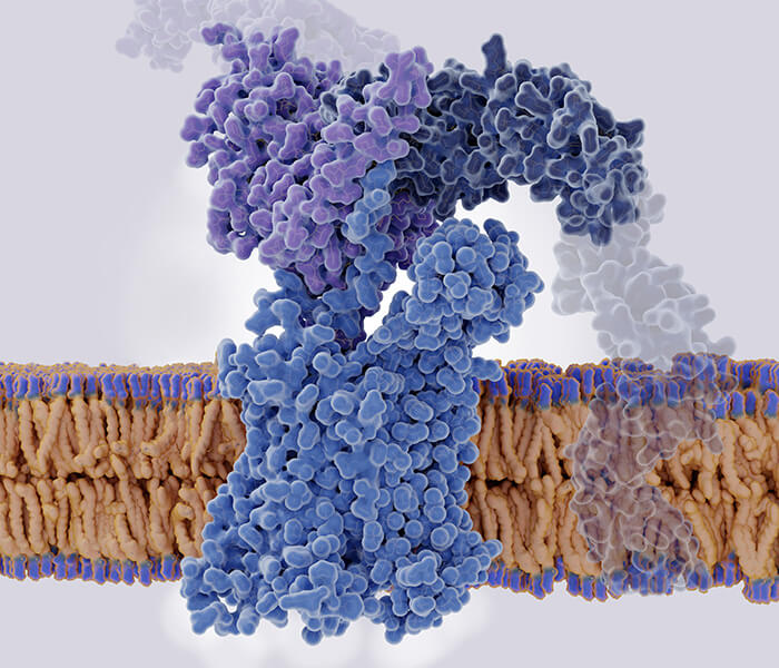
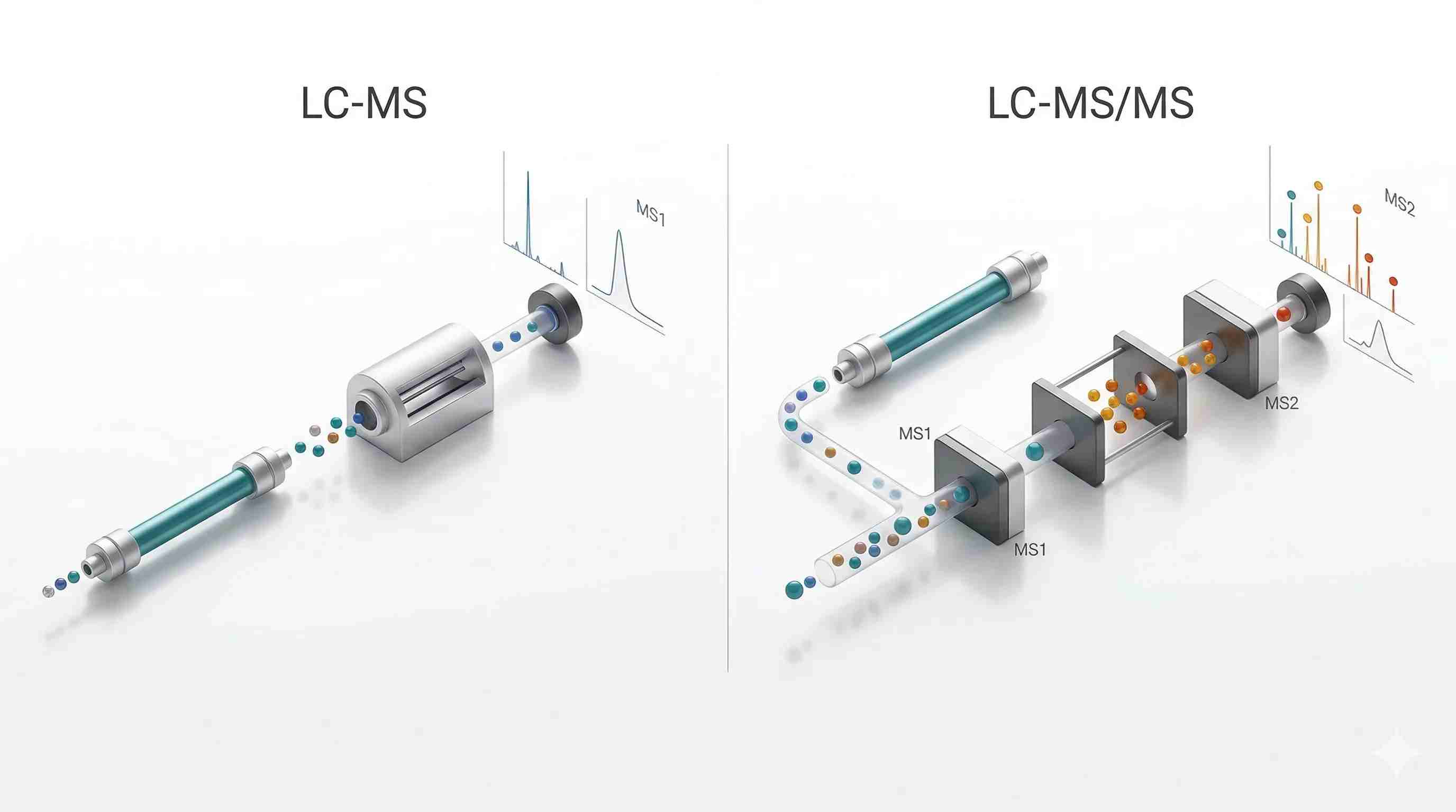 Figure 1. Multidimensional selectivity in LC-MS and LC-MS/MS
Single-stage LC-MS relies mainly on chromatographic separation plus precursor-level mass measurement, whereas LC-MS/MS adds precursor isolation, controlled fragmentation, and fragment-ion readout to remove ambiguity across multiple analytical dimensions.
Visual structure:
- Left panel: LC column, ion stream, one mass-selection event, MS1 spectrum
- Right panel: LC column, precursor isolation, fragmentation chamber, fragment-ion spectrum
- Shared bottom layer: chromatographic peaks to show that both workflows start from partially resolved elution
- Minimal labels only: LC-MS, LC-MS/MS, MS1, MS2
This is the right point to introduce the figure because the reader needs to see that tandem MS is not simply "more data-rich." It is more selective because it creates more opportunities to reject the wrong answer.
In practical terms, this is the difference between detection and characterization. A strong MS1 feature may show that something is present near the expected mass. A tandem experiment can test whether that selected ion breaks apart in a way that supports the proposed identity. In simple samples, that extra layer may feel unnecessary. In modern proteomics and metabolomics, it is often what makes the interpretation defensible.
The Evolution of Selectivity: Why MS1 Alone Stops Being Enough
The first reduction in complexity happens in the LC system, not in the mass analyzer. The chromatographic method spreads analytes across retention time according to their interaction with the stationary phase and mobile-phase program. That step is essential, but it is never absolute. In deep proteomic digests, many peptide precursors still cluster tightly within the same elution region. In metabolomics, compounds with very different structures can remain close in both retention time and m/z space. The mass spectrometer is therefore almost never working on a truly simple input.
Single-stage LC-MS addresses this complexity mainly through accurate mass measurement. In the right context, that is highly valuable. Exact mass narrows candidate space, supports elemental composition filtering, and enables broad untargeted feature discovery. In a clean standard mixture or an early-stage exploratory run, that may be sufficient. This is one reason LC-MS remains central in discovery science.
The problem begins when accurate mass is treated as structural proof. Exact mass is a strong constraint, but it is not a unique fingerprint. Structural isomers can share the same formula. Unrelated compounds can fall into the same nominal mass region. Adduct formation can complicate interpretation. Co-eluting background ions can distort low-level signals. Source-derived fragments can masquerade as authentic low-mass species. In all of these cases, the MS1 layer appears precise while still leaving room for the wrong molecular story.
That is the true limitation of LC-MS in complex omics work. It provides good precursor-level evidence, but weak conditional evidence. It records what arrived at the detector. It does not force the ion to reveal how it behaves under controlled activation.
LC-MS/MS adds that missing interrogation step. A precursor ion is selected. It is then fragmented in a defined collision environment. The fragment ions are measured and interpreted. This turns one mass observation into a sequence of selective tests. Retention behavior narrows the search in time. Precursor isolation narrows the search in m/z. Fragmentation introduces structure-sensitive behavior. Fragment-ion detection tests whether the observed breakdown pattern matches a chemically plausible identity.
This is why tandem MS is best understood as a system of multidimensional selectivity. No single layer is perfect. Together, they remove different classes of ambiguity. That is the foundation of its power.
Why LC-MS Still Deserves a Central Place
A serious comparison must avoid the lazy conclusion that LC-MS is merely a preliminary or inferior form of mass spectrometry. That is not analytically correct.
LC-MS remains the right tool for many questions because not every experiment benefits from spending time on fragmentation. If the primary goal is broad feature inventory, exact-mass confirmation, rapid survey scanning, or intact-mass observation, MS1-focused acquisition may be the best use of instrument time. In untargeted screening, that can be especially valuable. A survey-first workflow can map chemical space efficiently before the analyst commits acquisition time to deeper characterization.
This is not just a philosophical point. It is a timing issue. Every acquisition method operates within a finite scan budget. Each added MS/MS event consumes time that could have been used to revisit another eluting peak. If the gradient is short and the peaks are narrow, that budget becomes tight very quickly. A pure MS1 method often samples the chromatographic profile more frequently because it avoids precursor isolation and collision steps. In some discovery settings, that can improve feature completeness at the survey layer.
Still, broad coverage is not the same as high-confidence interpretation. A method can observe many features while leaving a large fraction of them only weakly resolved in structural terms. That is the central trade-off. LC-MS often wins on survey efficiency. LC-MS/MS often wins on discrimination.
The boundary is practical. If the study needs a first-pass inventory, LC-MS may be the efficient front end. If the study needs structural confirmation, peptide-level identity support, interference-resistant quantification, or strong control over false assignments, tandem MS becomes much harder to avoid. The method choice should therefore be driven by the type of error the experiment can tolerate, not by the appeal of collecting more or less data.
The Physics of Tandem MS: Why Fragmentation Is the Real Information Step
Many articles introduce MS/MS as if fragmentation were a routine middle stage between two scans. That description misses the most important point. Fragmentation is where the experiment stops being purely observational and becomes mechanistic.
A precursor ion is not just measured in tandem MS. It is challenged. Energy is deposited into it. Bonds redistribute strain. Some cleavage pathways become favorable. Others do not. The resulting spectrum is therefore not simply a list of product-ion masses. It is the outcome of how a selected molecular ion responded to a defined activation environment.
This matters because different analytical goals require different fragmentation behavior.
In proteomics, the analyst needs fragment ions that support peptide sequence interpretation. Too little fragmentation yields sparse evidence. Too much fragmentation can spread signal across many weak ions and reduce interpretability. In metabolomics, the same principle appears in another form. The analyst may need substructural clues, characteristic neutral losses, or fragment patterns that strengthen library matching. Some compounds reward broad fragmentation. Others become less informative when the collision regime is too aggressive.
That is why tandem MS should never be reduced to "MS1 plus extra sensitivity." Its real value is structure-responsive fragmentation under controlled conditions. Without that, the method remains close to mass measurement. With that, it becomes molecular interrogation.
A useful way to think about tandem MS is as a three-part logic chain:
- Selection — isolate the precursor of interest
- Activation — deposit energy in a controlled collision environment
- Readout — measure the fragment population with enough selectivity to interpret it
If any one of these steps is weak, the final spectrum may still look busy while saying very little.
CID vs. HCD: Collision Regime Changes What the Molecule Can Tell You
CID and HCD are often introduced through short definitions. CID is described as lower-energy fragmentation. HCD is described as higher-energy fragmentation. That summary is not wrong, but it is not deep enough to guide real interpretation.
The more useful question is how ions experience the collision environment and how that environment changes fragment production.
CID, in its conventional form, transfers energy through ion-neutral collisions in a way that often favors gradual internal energy build-up. Fragmentation can be highly useful, but its behavior depends strongly on precursor chemistry, charge state, activation time, and the specific analyzer configuration. CID does not simply break an ion apart. It shapes which dissociation pathways become visible enough to measure.
HCD changes that environment. It is associated with beam-type collision behavior and often generates richer fragment populations, especially in Orbitrap-centered workflows. In peptide analysis, that can increase sequence-informative coverage and support stronger downstream identification or targeted confirmation. In practical terms, HCD often yields spectra that are better suited to modern high-resolution database searching and fragment-centric validation.
But richer fragmentation is not automatically superior. Some analytes benefit from broader fragment coverage because additional product ions improve confidence. Others become harder to interpret when intensity is distributed too widely or when fragile diagnostic ions lose prominence. This is especially important in metabolomics. A small change in collision regime can alter relative fragment intensities enough to affect library matching, isomer discrimination, and confidence in annotation. The same precursor can look highly informative under one setting and only moderately useful under another.
This is why collision energy should not be inherited blindly from an older method file. Fragmentation behavior is context-dependent. It depends on analyte class, precursor stability, matrix complexity, isolation purity, and the purpose of the experiment. The best spectrum is not the busiest spectrum. It is the one that preserves the most discriminating information.
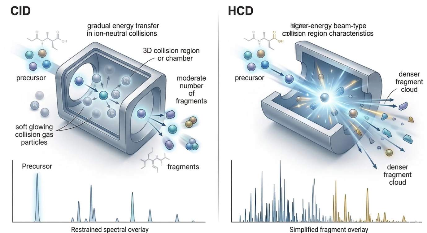 Figure 2. CID vs HCD collision physics and fragment coverage
CID and HCD are both collision-based fragmentation modes, but they differ in how energy is deposited and in the kinds of fragment populations they tend to emphasize, which changes spectral interpretability in both peptide and small-molecule analysis.
Visual structure:
- Left panel: CID chamber with gradual energy transfer and a moderate fragment population
- Right panel: HCD chamber with beam-type higher-energy activation and broader fragment output
- Bottom overlay: simplified product-ion spectra to show relative coverage differences
- Restricted labels only: CID, HCD, precursor, fragments
The figure is placed here because the reader now needs to connect fragmentation mode to analytical consequence. The point is not that one mode is universally better. The point is that collision regime determines what kind of structural evidence becomes visible.
SRM and MRM: Why the Double Filter Still Defines Targeted Sensitivity
When researchers describe the exceptional sensitivity of triple quadrupole assays, they are usually describing the success of SRM or MRM. The reason these methods remain so powerful is straightforward. They do not rely on one selective event. They rely on two.
First, the precursor ion must match the selected m/z in the first quadrupole. Then, after fragmentation, one chosen product ion must match the selected m/z in the third quadrupole. Signal is accepted only if both filters are passed in sequence. This is why SRM and MRM remain so effective in complex matrices. Many background ions can survive one filter. Far fewer survive two when the transition is well chosen.
That filtering logic is more important than simple ion count. A method can perform extremely well not because it records the largest amount of raw signal, but because it rejects irrelevant signal so effectively that the target trace becomes clean and easy to integrate. In practical assays, background suppression often matters as much as detector sensitivity.
This is why transition design is not a minor optimization step. It is the analytical core of the assay. A strong transition begins with a precursor that is selective enough in the real matrix. It then relies on a product ion that is both abundant and discriminating. If the precursor is too crowded, the first filter leaks interference. If the fragment is too generic, the second filter stops protecting specificity. If the collision energy is poorly set, the fragment may be present but not strong enough for stable quantification.
Good MRM method development therefore starts with questions of selectivity rather than convenience:
- Is the precursor sufficiently unique under the expected chromatographic conditions?
- Is the fragment abundant enough to support repeatable integration?
- Is the fragment structurally informative rather than merely intense?
- Does the transition remain clean across the real retention window of the analyte?
These questions matter in both proteomics and metabolomics. In peptide assays, shared sequence motifs and complex digests can create transition interference if fragment choice is careless. In small-molecule assays, adduct behavior, matrix suppression, and source chemistry can make a transition look elegant in a standard while turning messy in a biological extract. The transition has to encode true selectivity, not just nominal sensitivity.
In workflows that need focused targeted quantification, this is exactly where SRM & MRM becomes relevant. The value is not that the acronym sounds specialized. The value is that a well-designed double-filter workflow can reduce chemical background so aggressively that low-level targets become quantitatively tractable.
Duty Cycle: The Constraint That Quietly Controls Method Quality
Transition quality alone does not guarantee assay quality. The hidden variable is duty cycle.
Every targeted LC-MS/MS method operates within a fixed time budget. The instrument has to monitor all required transitions while the analyte is eluting. If too many transitions are active at the same time, dwell time per transition falls. If cycle time becomes too long relative to chromatographic peak width, too few data points are collected across the peak. Once that happens, integration becomes less stable, quantitative precision declines, and retention-time drift becomes more damaging.
This is not a minor tuning issue. It is one of the main reasons a method can look excellent in a sparse test mix and then lose performance in a real multiplexed panel.
The reason is simple. Chromatography and acquisition design are tightly coupled. Narrow peaks require fast revisit rates. Broad peaks are more forgiving. Short gradients compress more analytes into the same time region, which increases the number of concurrent transitions competing for the same cycle-time budget. Longer gradients spread analytes more gently across time, which often reduces competition and improves quantitative stability.
This leads to three practical method-design rules.
First, extend the gradient when co-elution pressure is the main reason targets are competing inside the same acquisition window. A longer gradient does not magically improve sensitivity, but it often improves effective selectivity by lowering local congestion.
Second, reduce concurrent transitions when the assay already has acceptable analyte coverage but unstable peak integration. Watching too many transitions poorly is usually worse than watching slightly fewer transitions well.
Third, prefer scheduled MRM over simply widening monitoring windows when chromatography is stable enough to support retention-time prediction. Scheduled monitoring preserves cycle-time efficiency by allowing the instrument to focus on transitions that are actually likely to be eluting. Broad windows are safer against retention drift, but they spend more of the duty-cycle budget on time periods where no useful signal is expected.
These are not abstract guidelines. They are the practical boundary between a method that detects a target and a method that quantifies it well.
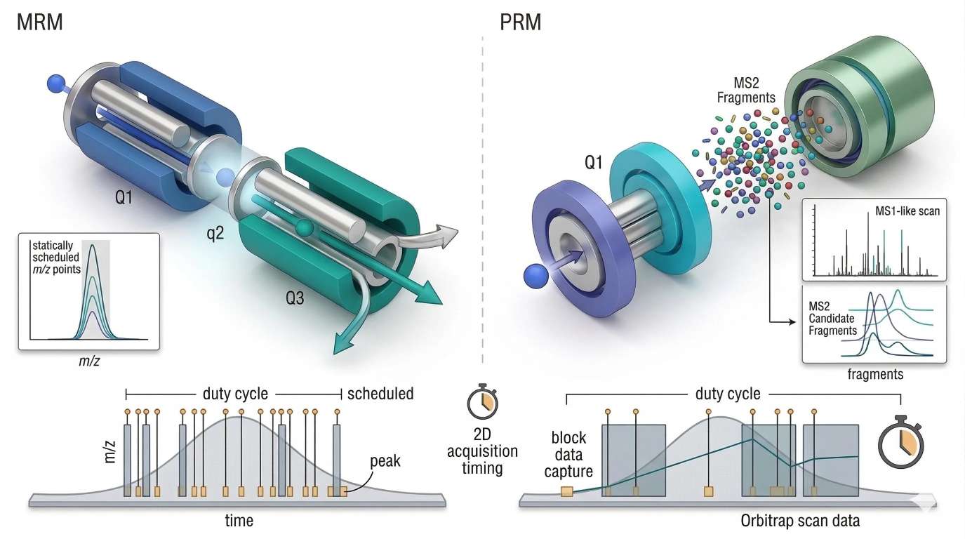 Figure 3. MRM vs PRM with duty cycle and transition scheduling
In targeted LC-MS/MS, analytical quality depends not only on transition selectivity but also on how the finite acquisition budget is distributed across eluting peaks, scheduled windows, and scan events.
Visual structure:
- Left panel: MRM on a triple quadrupole with precursor filter, collision cell, product-ion filter
- Right panel: PRM with precursor isolation followed by high-resolution full-fragment readout
- Lower strip: chromatographic peak width, sampling points, scheduled windows, cycle-time budget
- Minimal labels only: MRM, PRM, duty cycle, scheduled
The figure is inserted here because duty cycle is easier to grasp once the reader sees peak width and acquisition pressure together. Each transition or scan event costs time. Each narrowing of the chromatographic peak increases the need for rapid revisits.
PRM: A Different Answer to the Targeted Analysis Problem
PRM became attractive because it changes where selectivity is applied. Instead of monitoring only a small predefined set of product ions one by one, PRM isolates the precursor, fragments it, and records a richer high-resolution fragment population in a single event. That shifts the advantage from rigid preselection toward post-acquisition flexibility.
This is especially useful in complex proteomics. If one fragment ion turns out to be interfered, another may still be available in the data. The analyst is not forced to commit every fragment choice before the sample is acquired. High-resolution fragment measurement also adds confidence when the background is complex and when low-resolution product-ion overlap would weaken interpretation.
That flexibility explains why Parallel Reaction Monitoring (PRM) is often a strong fit for peptide-focused targeted studies that need both confidence and adaptability at the fragment level. The attraction is not simply high resolution. It is the ability to preserve a broader fragment record while still keeping the analysis targeted.
But PRM does not erase duty-cycle constraints. It redistributes them.
Capturing a full fragment population requires scan resources. In highly multiplexed assays, under short gradients, or across very narrow peaks, the same time-budget pressure still applies. Triple quadrupoles remain dominant in many ultra-sensitive targeted assays for a reason. Their logic is optimized for fast, focused, low-background transition monitoring. PRM offers more fragment evidence and more flexibility, but it is not a universal replacement for carefully optimized MRM.
The better way to compare them is not to ask which platform is more modern. It is to ask where the workflow should carry the burden of selectivity.
MRM places more of that burden before and during acquisition.
PRM preserves more options after acquisition.
That distinction becomes even more important in the second half of the article, where targeted monitoring gives way to broader acquisition strategies. Once the system is no longer following a defined transition list, duty cycle stops being a quiet design parameter and becomes one of the main forces that determines data completeness itself.
Data-Dependent Acquisition vs. Data-Independent Acquisition: Two Ways to Spend the Same Time Budget
Targeted assays tell the instrument what to watch. Discovery workflows do not have that luxury. The system has to decide how to distribute attention before the analyst knows which molecules will matter most. That is where DDA and DIA diverge.
Data-dependent acquisition is built on competitive selection. The instrument records an MS1 survey scan, ranks precursor ions by intensity or related rules, and then fragments the top candidates in that cycle. The logic is efficient. Stronger precursors are more likely to produce useful MS/MS spectra, so the system spends its time where it expects the greatest return.
In moderate-complexity samples, this works well. The instrument isolates a manageable set of precursors, generates relatively clean tandem spectra, and supports confident downstream searching. That is one reason DDA became the dominant engine of discovery proteomics for so long. It produces spectra that are often easy to interpret because each MS/MS event is tied to a selected precursor rather than to a broad mixed window.
The weakness appears when precursor density rises faster than duty cycle can keep up. In a deep proteomic digest, many peptide ions occupy the same retention window. In a complex metabolomics extract, chemically distinct species compete within narrow RT and m/z neighborhoods. The instrument cannot fragment all of them. It has to choose. Once the Top-N quota is filled, lower-abundance precursors are deferred. If they elute quickly, overlap with stronger neighbors, or sit near the edge of the sampling window, they may never be selected at all.
That is the real source of many missing values in DDA. The issue is not always that a peptide or metabolite failed to ionize. Often it was visible at MS1 level but lost the competition for MS/MS time. A precursor can therefore be chemically present and still disappear from the tandem layer in one run while being successfully fragmented in another. DDA does not fail because it produces poor spectra. It fails, in crowded samples, because it cannot visit every meaningful precursor with equal consistency.
DIA starts from a different assumption. Instead of asking which ions deserve fragmentation, it fragments ions systematically across predefined m/z windows during the whole chromatographic run. This changes the bias structure of the experiment. Lower-abundance ions no longer depend entirely on winning a Top-N race at the right moment. In principle, much more of the sample leaves a digital fragment record.
That is why DIA often improves completeness and run-to-run consistency. In large-scale quantitative proteomics, that advantage is especially important. A workflow that samples a wider fraction of the precursor space more systematically can reduce stochastic precursor loss and improve cross-sample comparability. This is also why DIA Quantitative Proteomics Service and 4D-DIA Quantitative Proteomics Service fit studies where reproducible quantitative coverage matters as much as raw identification count.
But DIA does not escape physics. It relocates the bottleneck. DDA often misses ions because they were never fragmented. DIA fragments far more of the sample, but many precursors are co-fragmented within the same isolation window. The resulting MS/MS record is chimeric. The problem has shifted from precursor selection to signal disentanglement. The analyst is no longer asking only, "Was this precursor selected?" The harder question becomes, "Can this mixed fragment population be correctly deconvolved into the right precursor-fragment relationships?"
This is why DDA and DIA should not be described as old versus new, or as simple versus advanced. They are two different ways to spend the same finite acquisition budget.
DDA spends more time on selective interrogation.
DIA spends more time on systematic coverage.
DDA often gives cleaner precursor-linked spectra, but it can miss lower-abundance signals.
DIA often gives a more complete digital record, but it demands much stronger computational separation after acquisition.
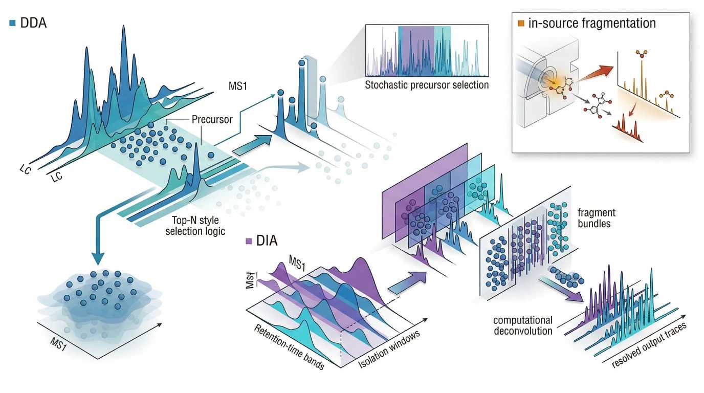 Figure 4. DDA vs DIA acquisition logic and in-source fragmentation artifact
DDA prioritizes selected precursors for cleaner tandem spectra, whereas DIA fragments precursor populations more systematically at the cost of greater spectral mixing; both strategies can still be complicated by source-generated artifacts that distort the precursor story before intentional MS/MS begins.
Visual structure:
- Left panel: DDA Top-N selection with some low-abundance precursors bypassed
- Right panel: DIA window-based fragmentation with dense mixed fragment populations and downstream deconvolution
- Corner inset: in-source fragmentation event producing misleading low-mass ions before formal MS/MS
- Minimal labels only: DDA, DIA, in-source fragmentation
The figure belongs here because the reader now needs to see that acquisition strategy is really a decision about where ambiguity will be managed: before fragmentation, after fragmentation, or partly in both places.
The Real Variable Behind DDA and DIA Performance: Duty Cycle Meets Chromatographic Peak Width
Many summaries of DDA versus DIA stop at workflow definitions. That leaves out the most important practical point: acquisition mode only makes sense in the context of chromatographic timing.
Every LC-MS/MS method lives inside a time budget. The instrument has only a limited number of analytically meaningful actions it can perform while a chromatographic peak is still eluting. Broad peaks are forgiving because they allow more revisit opportunities. Narrow peaks are unforgiving because the instrument has fewer chances to inspect that signal before it disappears. This is why gradient length matters so much. It is not just a separation variable. It is a sampling variable.
In DDA, short gradients and narrow peaks amplify competition. Many precursors co-elute inside compressed time windows, and the Top-N list becomes more exclusionary by necessity. Strong ions dominate repeatedly. Lower-abundance species may appear clearly in MS1 but never receive MS/MS attention. A longer gradient can reduce that pressure by spreading precursor populations across time, lowering local congestion and increasing the probability that weaker precursors will be sampled.
In DIA, the same compression problem appears in another form. The workflow no longer depends on competitive Top-N selection, but it still has to cycle through all DIA windows fast enough to sample each peak adequately. If the full window set takes too long, points across the peak fall. If the windows are too broad, spectral mixing becomes more severe. If the windows are too narrow, the cycle can become too slow. DIA is therefore not free from duty-cycle pressure. It simply converts that pressure into a window-design problem.
This is one of the central truths of modern LC-MS/MS: chromatography and acquisition cannot be optimized independently.
A longer gradient often improves precursor distribution, lowers local crowding, and gives both DDA and DIA more room to behave well. But longer gradients reduce throughput. Shorter gradients increase throughput, but they force harsher compromises. In DDA, that usually means shallower sampling of lower-level precursors. In DIA, that often means wider windows, denser chimeric spectra, or fewer sampling points across each peak.
That is why method planning should begin with the sample and the decision goal, not with platform loyalty. If the sample is extremely complex and the study depends on consistent quantitative coverage across many runs, DIA may justify the burden of downstream deconvolution. If the sample is cleaner or the main priority is high-quality precursor-linked tandem spectra, DDA may still be the more efficient architecture. The right choice is the one that spends acquisition time where the experiment removes the most ambiguity.
In-Source Fragmentation: The Hidden Artifact That Can Mislead Both LC-MS and LC-MS/MS
One of the most underestimated problems in omics MS is that fragmentation does not always begin where the analyst thinks it begins.
In-source fragmentation occurs when ions undergo partial breakdown in or near the ion source before deliberate MS/MS activation. This can happen because of source voltage, desolvation stress, transfer conditions, analyte instability, or matrix-dependent effects. The consequence is subtle but serious. Source-generated fragments can appear as if they were independent analytes, plausible low-mass metabolites, or authentic precursor species.
This problem is especially dangerous in metabolomics. Many small molecules are chemically labile, and annotation often starts from feature-level reasoning. A source fragment can co-elute with its parent, carry a plausible m/z, and survive early filtering steps. If the analyst leans too heavily on exact mass and retention behavior, that fragment can be mistaken for a biologically real metabolite rather than a product of ion formation.
Proteomics is not immune. Labile modifications, unstable precursor populations, and source-induced losses can all distort precursor purity or complicate downstream interpretation. In modified peptide analysis, what looks like a low-level independent species may actually reflect pre-fragmentation chemistry rather than a true analyte population in solution.
This is why "the instrument detected it" should never be treated as the end of the story. Detection does not reveal whether the ion originated as an intact molecule, an adduct, a neutral-loss derivative, or a source-generated fragment. Tandem MS helps, but it does not automatically solve the problem. If a source-derived fragment is isolated and fragmented again, the resulting MS/MS spectrum may still look coherent. The spectrum can be internally consistent while remaining anchored to the wrong precursor history.
The right response is not to distrust LC-MS/MS. It is to use it more critically. Source conditions should be optimized with analyte stability in mind. Co-elution between parent-like ions and fragment-like ions should be examined carefully. Collision-based confirmation should be interpreted alongside plausible source chemistry rather than in isolation. When a feature appears important but chemically suspicious, the correct question is not only "Does it fragment well?" but also "Did it enter the mass analyzer as the molecule we think it was?"
For untargeted small-molecule studies, this is one reason why LC-MS/MS Untargeted Metabolomics, Targeted Metabolomics, and Unknown Metabolites Identification often require different validation logic even when they are run on related platforms. The challenge is not just generating spectra. It is deciding how much of the spectral story belongs to the actual analyte and how much belongs to source and acquisition behavior.
LC-MS vs. LC-MS/MS in Proteomics: When the Advantage Becomes Decisive
Proteomics makes the limitations of single-stage MS especially visible because peptide identification is not just a mass-matching exercise. Even when mass accuracy is excellent, many peptides remain ambiguous at the precursor level. Shared compositions, near-isobaric species, co-elution, charge-state complexity, and post-translational modifications all increase the interpretive burden. A peptide feature without fragment support may still be suggestive, but it rarely carries the same weight as a sequence-supported tandem event.
This is why LC-MS/MS became the central engine of bottom-up proteomics. The experiment does not merely observe peptide precursors. It converts them into fragment patterns that can support sequence inference. Once fragments are recorded, the data become searchable against peptide databases, spectral libraries, or targeted transition logic. The workflow moves from mass observation to sequence-resolved evidence.
The advantage becomes even more decisive in quantification. In discovery proteomics, DDA and DIA determine how completely peptides are sampled across runs. In targeted proteomics, MRM and PRM determine how selectively and reproducibly peptide abundance can be tracked in complex backgrounds. In both cases, the central problem is the same: precursor mass alone is rarely enough when the matrix is crowded and the conclusion must survive replication.
That does not mean LC-MS has no role in proteomics. It remains useful for intact-mass observation, system suitability checks, survey runs, and selected specialized applications where sequence-level evidence is not the immediate goal. But when the claim depends on peptide identity, PTM-aware characterization, or interference-resistant quantification, tandem MS is the evidentiary core of the workflow.
That is also why Proteomics Service, Protein Identification Services, and Shotgun Protein Identification sit on one side of the decision space, while Parallel Reaction Monitoring (PRM) and SRM & MRM sit on another. The dividing line is not whether MS is being used. It is whether the experiment is asking for broad discovery, targeted confirmation, or quantitative control under interference.
LC-MS vs. LC-MS/MS in Metabolomics: Why Structural Confidence Is the Hardest Currency
Metabolomics presents a different kind of difficulty. Peptides follow sequence logic. Small molecules do not. The chemical diversity is broader, fragmentation behavior is less uniform, and structural isomers often create harder annotation problems than peptide-centric workflows encounter. In this setting, accurate mass is useful but structurally incomplete.
Single-stage LC-MS remains essential in metabolomics because broad untargeted surveys depend on it. Feature discovery, exact-mass filtering, isotope inspection, and cross-group comparison often begin at the MS1 layer. That layer is efficient and information-rich. It is also easy to overinterpret.
A metabolite feature can look compelling for several reasons that have little to do with confirmed identity. It may match an expected exact mass. It may shift strongly between biological groups. It may sit within a pathway that makes biochemical sense. But unless tandem evidence strengthens the assignment, the interpretation can remain fragile. Isomers, adducts, in-source fragments, and background interferences all weaken the link between precursor mass and actual structure.
Adduct form is part of this problem. The same metabolite can enter the analyzer as different ionic species, and those ionic forms do not always fragment in equally useful ways. One adduct may yield a spectrum rich in diagnostic ions. Another may produce weaker or less interpretable fragmentation. That means the quality of structural evidence does not depend only on collision energy. It also depends on which ion form is being fragmented.
Collision energy then adds a second layer of complexity. In metabolomics, the best library match is not always produced by the highest-energy setting. Too little energy may leave the spectrum sparse. Too much energy may shift ion intensity away from the most diagnostic fragments or produce overly dense low-specificity patterns. Library scoring, isomer discrimination, and annotation confidence can therefore change substantially with collision regime even for the same precursor.
This is why annotation tier matters. Exact mass alone may support a provisional feature assignment, but higher-confidence structural interpretation usually requires MS/MS evidence, retention behavior, adduct-aware reasoning, and careful exclusion of source artifacts. In practice, when a metabolite signal looks important, the troubleshooting order should often be:
- rule out source-derived fragments and unstable adduct behavior,
- assess co-elution and matrix interference,
- optimize collision conditions for diagnostic rather than merely abundant fragments,
- then evaluate spectral matching or targeted confirmation.
That sequence is easy to ignore when the feature table is large and the biology is exciting. It should not be ignored. In metabolomics, the difference between an interesting feature and a defendable molecular interpretation is often the quality of tandem evidence.
Decision Framework: When Is LC-MS Enough, and When Does LC-MS/MS Become Necessary?
The table below summarizes dominant analytical tendencies rather than absolute performance claims, because matrix, acquisition design, and chromatographic context can shift the balance.
| Sample | Analytical goal | Better-fit architecture |
|---|---|---|
| Moderate-complexity extract | Broad feature inventory and rapid prioritization | LC-MS |
| Complex proteomic digest | Peptide identification with deeper sequence support | LC-MS/MS |
| Cohort-scale quantitative proteomics | Consistent cross-run sampling and data completeness | LC-MS/MS with DIA |
| Sparse targeted peptide panel | Maximum sensitivity and low-background quantification | LC-MS/MS with MRM/SRM |
| Targeted peptide verification in complex matrix | High-confidence fragment-level confirmation with flexibility | LC-MS/MS with PRM |
| Isomer-heavy small-molecule mixture | Stronger structural differentiation | LC-MS/MS |
| Short-gradient high-throughput screen | Efficient first-pass survey where structural certainty is secondary | LC-MS |
| Untargeted metabolite discovery followed by confirmation | MS1 survey first, then tandem validation on prioritized features | Combined LC-MS and LC-MS/MS |
The practical rule is simple. The more the study depends on rejecting plausible wrong answers, the more useful tandem MS becomes.
LC-MS is often enough when:
- the main goal is broad screening or feature inventory
- exact mass is being used for early prioritization rather than final identity claims
- the sample is relatively simple
- throughput matters more than structural confidence
- the study needs a fast survey layer before deeper follow-up
LC-MS/MS becomes difficult to avoid when:
- the matrix is complex
- the analyte is low in abundance
- structural isomers or close interferences are plausible
- the assay must tolerate substantial chemical background
- quantification has to be precise and reproducible
- peptide-level or fragment-level evidence is required
- metabolite annotation must move beyond feature-level plausibility
The right question is therefore not "Which platform is more powerful?" Both are powerful. The right question is "What kind of error can this workflow afford?" If the study can tolerate provisional feature-level evidence, LC-MS may be sufficient as a first analytical pass. If the study must defend identity, isolate trace analytes from noise, or quantify targets in crowded matrices, LC-MS/MS is usually the stronger architecture.
Comparison Table: LC-MS vs. LC-MS/MS
The table below summarizes dominant analytical tendencies rather than absolute performance claims, because matrix, acquisition design, and chromatographic context can shift the balance.
| Metric | LC-MS | LC-MS/MS |
|---|---|---|
| Core readout | Precursor-level mass information | Precursor plus fragment-ion information |
| Primary strength | Broad survey efficiency and accurate-mass profiling | Multidimensional selectivity and stronger confirmation |
| Dynamic range in complex samples | Often constrained by background and co-eluting interference | Often improved in practice because interference is rejected more effectively |
| Isomer resolution | Limited unless LC separation alone is sufficient | Stronger when fragmentation yields differentiating product ions |
| Sensitivity for trace metabolites | Good in cleaner systems, less robust in chemically crowded matrices | Typically stronger in targeted workflows because background is suppressed |
| Quantitative precision | Useful for broad profiling, but vulnerable to interference | Often better for targeted assays when cycle time and transitions are well optimized |
| Best fit in proteomics | Survey, intact-mass checks, selected specialized use cases | Identification, DDA, DIA, PRM, MRM, targeted quantification |
| Best fit in metabolomics | Untargeted feature discovery and exact-mass screening | Structural confirmation, targeted quantification, reduced annotation ambiguity |
| Main weakness | Mass alone rarely proves identity in complex samples | Greater method complexity and stronger dependence on acquisition design |
| Main hidden risk | Overconfidence in feature annotation | False confidence from poor precursor isolation, poor energy tuning, or source artifacts |
Final Perspective: Tandem MS Wins Not Because It Sees More, but Because It Tests More
The usual summary says LC-MS/MS is more selective, more sensitive, and more informative than LC-MS. That is true, but it still misses the deeper reason tandem workflows matter.
The real advantage is that LC-MS/MS turns mass spectrometry from a mainly observational tool into a conditional testing system. A precursor must be isolated. It must survive a defined collision regime. Its fragments must support a coherent interpretation. Each stage challenges a different class of wrong answer. That is why LC-MS/MS is so effective in modern proteomics and metabolomics. It does not merely collect more information. It subjects the information to more analytical scrutiny.
Single-stage LC-MS remains indispensable because broad surveying still matters. Many workflows should begin there. But when the sample is dense, the analyte is scarce, or the interpretation threshold is stringent, one mass filter is rarely enough. Modern omics does not usually fail because ions were invisible. It fails because ambiguity was underestimated.
That is the real lesson behind duty cycles, collision physics, and multidimensional selectivity. The best LC-MS/MS method is not the one with the longest feature list or the busiest spectra. It is the one that spends its finite acquisition budget where ambiguity is highest, and removes as much of that ambiguity as possible before the scientific conclusion is written.
FAQ
What is the main difference between LC-MS and LC-MS/MS?
LC-MS mainly measures precursor ions after chromatographic separation. LC-MS/MS adds a second stage in which a selected precursor is fragmented and the product ions are measured. That extra step provides stronger selectivity and much better support for structural or sequence-level interpretation.
Is LC-MS/MS always more sensitive than LC-MS?
Not in every abstract sense, but in complex samples it is often more effective for low-level targets because tandem workflows reject more background. In targeted assays such as MRM, the gain often comes from cleaner signal rather than simply from a larger ion count.
Why is LC-MS alone often not enough for metabolite identification?
Because exact mass narrows candidates but rarely proves structure on its own. Isomers, adducts, co-eluting interferences, and in-source fragments can all create misleading assignments. MS/MS adds fragment evidence that improves annotation confidence.
Why does proteomics rely so heavily on LC-MS/MS?
Because peptide identity usually depends on fragment-ion evidence. Precursor mass alone is rarely enough to assign sequences confidently in a complex digest. Tandem MS provides the fragment patterns needed for database searching, discovery workflows, and targeted quantification.
What is the practical advantage of MRM over PRM?
MRM usually offers very high sensitivity and low background through double mass filtering, which makes it excellent for focused targeted quantification. PRM offers greater post-acquisition flexibility because a fuller high-resolution fragment set is recorded after precursor isolation.
What is the main trade-off between DDA and DIA?
DDA often generates cleaner precursor-specific MS/MS spectra, but it can miss lower-abundance ions because precursor selection is competitive. DIA captures a more complete fragment record of the sample, but the spectra are more mixed and require stronger computational deconvolution.
Why does gradient length affect LC-MS/MS performance?
Because gradient length influences peak width and local analyte crowding. Narrower peaks and shorter gradients compress more events into a smaller time window, which increases pressure on duty cycle and can reduce sampling quality in both DDA and DIA.
What is in-source fragmentation, and why is it dangerous?
It is fragmentation that occurs in or near the ion source before deliberate MS/MS activation. It is dangerous because the resulting ions can be mistaken for authentic analytes or meaningful precursor species, especially in untargeted workflows.
References
- Bekker-Jensen, D. B., Martínez-Val, A., Steigerwald, S., et al. 2020. A compact quadrupole-Orbitrap mass spectrometer with FAIMS interface improves proteome coverage in short LC gradients. Molecular & Cellular Proteomics, 19(4), 716–729. DOI: 10.1074/mcp.TIR119.001906
- Searle, B. C., Swearingen, K. E., Barnes, C. A., et al. 2020. Generating high-quality libraries for DIA MS with empirically corrected peptide predictions. Nature Communications, 11, 1548. DOI: 10.1038/s41467-020-15346-1
- Ludwig, C., Gillet, L., Rosenberger, G., Amon, S., Collins, B. C., & Aebersold, R. 2018. Data-independent acquisition-based SWATH-MS for quantitative proteomics: a tutorial. Molecular Systems Biology, 14(8), e8126. DOI: 10.15252/msb.20178126
- Bruderer, R., Bernhardt, O. M., Gandhi, T., Miladinović, S. M., Cheng, L. Y., Messner, S., Ehrenberger, T., Zanotelli, V., Butscheid, Y., Escher, C., Vitek, O., Rinner, O., Reiter, L., & Aebersold, R. 2015. Extending the limits of quantitative proteome profiling with data-independent acquisition and application to acetaminophen-treated three-dimensional liver microtissues. Molecular & Cellular Proteomics, 14(5), 1400–1410. DOI: 10.1074/mcp.M114.044305
- Gallien, S., Kim, S. Y., & Domon, B. 2015. Large-scale targeted proteomics using internal standard triggered-parallel reaction monitoring (IS-PRM). Molecular & Cellular Proteomics, 14(6), 1630–1644. DOI: 10.1074/mcp.O114.043968
- Peterson, A. C., Russell, J. D., Bailey, D. J., Westphall, M. S., & Coon, J. J. 2012. Parallel reaction monitoring for high resolution and high mass accuracy quantitative, targeted proteomics. Molecular & Cellular Proteomics, 11(11), 1475–1488. DOI: 10.1074/mcp.O112.020131
- Gallien, S., Duriez, E., & Domon, B. 2011. Selected reaction monitoring applied to proteomics. Journal of Mass Spectrometry, 46(3), 298–312. DOI: 10.1002/jms.1904
- Hu, A., Noble, W. S., & Wolf-Yadlin, A. 2016. Technical advances in proteomics: new developments in data-independent acquisition. F1000Research, 5, 419. DOI: 10.12688/f1000research.7042.1
- Röst, H. L., Rosenberger, G., Navarro, P., Gillet, L., Miladinović, S. M., Schubert, O. T., Wolski, W., Collins, B. C., Malmström, J., Malmström, L., & Aebersold, R. 2014. OpenSWATH enables automated, targeted analysis of data-independent acquisition MS data. Nature Biotechnology, 32, 219–223. DOI: 10.1038/nbt.2841
- Lou, R., Wang, R., Wei, X., Jia, Z., Yang, Z., Li, K., Zheng, H., Li, Y., Wang, Y., Luo, J., Wu, H., Yuan, J., & Xu, Y. 2024. The hidden impact of in-source fragmentation in metabolic and chemical mass spectrometry data interpretation. Nature Metabolism, 6, 1018–1031. DOI: 10.1038/s42255-024-01076-x
- Zhang, Y., Fonslow, B. R., Shan, B., Baek, M.-C., & Yates, J. R. 2013. Protein analysis by shotgun/bottom-up proteomics. Chemical Reviews, 113(4), 2343–2394. DOI: 10.1021/cr3003533