Phosphoproteomics, the field focused on protein phosphorylation, is essential for deciphering cellular signaling and regulatory pathways. Computational biologists analyzing such data demand specialized approaches to manage its scale and complexity, extracting meaningful mechanistic insights. This paper details a systematic methodology employing R and bioinformatics resources for phosphoproteomic analysis, emphasizing critical techniques, relevant software packages, and efficient workflows.
Applicable tools: R (4.0+), Bioconductor, Perseus, Python (optional).
Input data: quantitative matrix of phosphorylation sites (Phospho (STY)Sites.txt) output by MaxQuant/DIA-NN.
1. Data preprocessing and quality control
1.1 Data Loading and Filtering
r
library(tidyverse)
library(phosphonets)
# Load MaxQuant/DIA-NN output files
phospho_data <- read_tsv("Phospho_(STY)Sites.txt",
col_types = cols(.default = "c",
Intensity = "d",
Localization.prob = "d"))
# Strict filtering criteria
filtered_data <- phospho_data %>%
filter(Localization.prob >= 0.75) %>% # Retain high-confidence sites
filter(!grepl("REV_|CON__", Proteins)) %>% # Remove reverse database hits and contaminants
filter(Score > 40) %>% # Threshold for mass spectrometry identification score
select(Protein, Position, Amino.acid,
contains("Intensity"), Sequence)
1.2 Missing Value Imputation Strategies
| Method | Applicable Scenario | R Code |
|---|---|---|
| Random Forest Imputation | Missing rate > 30% | impute::missForest(phospho_matrix) |
| KNN Imputation | Missing rate 15-30% | impute::impute.knn(phospho_matrix, k=10) |
| Minimum Value Imputation | Missing rate < 15% | apply(phospho_matrix, 2, function(x) ifelse(is.na(x), min(x, na.rm=T), x)) |
1.3 Batch Effect Correction
r
library(sva)
# Create design matrix
design <- model.matrix(~ group) # 'group' represents experimental conditions
# ComBat correction
corrected_data <- ComBat(
dat = as.matrix(log2(phospho_matrix)),
batch = batch_vector, # Batch information vector
mod = design,
par.prior = TRUE
)
2. Differential Phosphorylation Analysis
2.1 Limma Differential Analysis
r
library(limma)
# Create contrast matrix
contrast.matrix <- makeContrasts(
Tumor_vs_Normal = Tumor - Normal,
levels = design
)
# Linear model fitting
fit <- lmFit(corrected_data, design) %>%
contrasts.fit(contrast.matrix) %>%
eBayes()
# Extract results
diff_results <- topTable(
fit,
coef = "Tumor_vs_Normal",
number = Inf,
p.value = 0.05,
lfc = 1 # log2 fold-change threshold
)
2.2 Phosphorylation Site-Specific Analysis
r
# Extract phosphosite context sequences
diff_results <- diff_results %>%
mutate(
motif_15mer = str_sub(Sequence, start = -7, end = 7),
site_id = paste0(Gene.names, "_", Amino.acid, Position)
)
# Kinase-substrate enrichment analysis
library(PhosR)
kinase_enrich <- kinaseSubstrateEnrichment(
diff_results$site_id,
species = "human",
method = "Fisher"
)
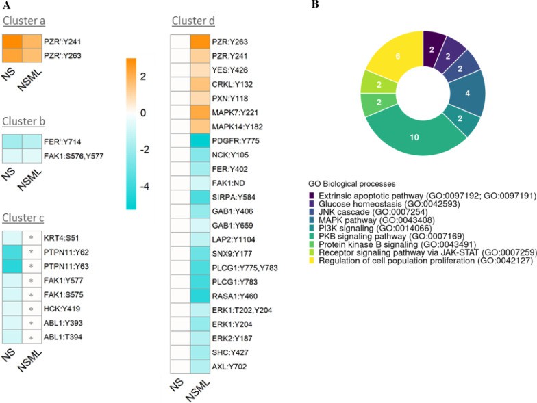 Analysis of dysregulated phosphosites in RASopathy interactome proteins in NS, NSML (Montero-Bullón JF et al., 2021)
3. Functional Annotation and Pathway Enrichment
3.1 Kinase Activity Prediction
r
# Calculate kinase activity using phosphosite data
kinase_activity <- computeKinaseActivity(
psite_data = diff_results,
species = "human",
id_type = "site_id",
method = "linear"
)
# Filter significant activity kinases
significant_kinases <- kinase_activity %>%
filter(p.adjust < 0.05, abs(activity_score) > 1.5)
3.2 Pathway Enrichment Analysis
r
library(clusterProfiler)
library(org.Hs.eg.db)
# Gene ID conversion
entrez_ids <- bitr(
diff_results$Gene.names,
fromType = "SYMBOL",
toType = "ENTREZID",
OrgDb = org.Hs.eg.db
)
# KEGG pathway enrichment
kegg_result <- enrichKEGG(
gene = entrez_ids$ENTREZID,
organism = "hsa",
pvalueCutoff = 0.05,
pAdjustMethod = "BH"
)
# Visualization
dotplot(kegg_result, showCategory=15, font.size=8)
4. Advanced Analysis Techniques
4.1 Phosphorylation Signaling Network Modeling
r
library(igraph)
# Build kinase-substrate interaction network
kinase_substrate_net <- kinaseSubstrateNetwork(
kinase_activity = significant_kinases,
substrate_data = diff_results,
correlation_threshold = 0.7
)
# Network topology analysis
network_metrics <- data.frame(
degree = degree(kinase_substrate_net),
betweenness = betweenness(kinase_substrate_net)
)
# Export to Cytoscape format
write_graph(kinase_substrate_net, "kinase_network.graphml", format = "graphml")
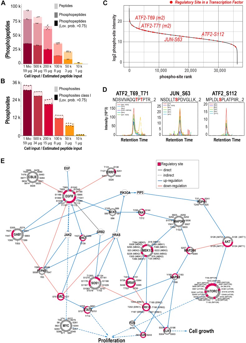 Enrichment and signal network construction (Bortel P et al., 2024)
4.2 Multi-omics Integrative Analysis
r
library(MOFA2)
# Create multi-omics object
mofa_object <- create_mofa(
data = list(
phosphoproteomics = t(phospho_matrix),
transcriptomics = t(rna_matrix),
proteomics = t(protein_matrix)
),
groups = sample_groups
)
# Model training
model <- run_mofa(
mofa_object,
n_factors = 10,
convergence_mode = "slow"
)
# Factor-feature association visualization
plot_weights(model, view = "phosphoproteomics", nfeatures = 10)
5. Visualization Techniques
5.1 Phosphorylation Heatmap
r
library(ComplexHeatmap)
library(circlize)
# Create annotation
ha <- HeatmapAnnotation(
Group = sample_groups,
col = list(Group = c("Tumor" = "red", "Normal" = "blue"))
)
# Generate heatmap
Heatmap(
as.matrix(diff_phospho_matrix),
name = "log2(Intensity)",
col = colorRamp2(c(-2, 0, 2), c("blue", "white", "red")),
top_annotation = ha,
show_row_names = FALSE,
row_km = 4, # Row clustering
column_km = 2 # Column clustering
)
5.2 Kinase Activity Bubble Plot
r
ggplot(significant_kinases,
aes(x = reorder(Kinase, activity_score),
y = activity_score)) +
geom_point(aes(size = -log10(p.value), color = Regulation)) +
scale_color_manual(values = c(down = "blue", up = "red")) +
coord_flip() +
labs(x = "Kinase", y = "Activity Score",
title = "Differential Kinase Activity") +
theme_minimal()
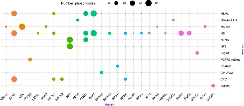 Bubble diagram of phosphorylation site of protein (Montero-Bullón JF et al., 2021)
6. Reproducibility Assurance
6.1 Docker Container Configuration
dockerfile
# Dockerfile
FROM rocker/rstudio:4.2.0
RUN apt-get update && apt-get install -y \
libxml2-dev \
libssl-dev \
libcurl4-openssl-dev
RUN R -e "install.packages(c('tidyverse', 'limma', 'phosphonets', 'clusterProfiler'))"
RUN R -e "BiocManager::install(c('org.Hs.eg.db', 'MOFA2'))"
COPY analysis_script.R /home/rstudio/
WORKDIR /home/rstudio
6.2 Snakemake Workflow Management
python
# Snakefile
rule all:
input: "results/final_report.html"
rule preprocess:
input: "data/Phospho_STY.txt"
output: "processed/filtered_data.rds"
script: "scripts/01_preprocessing.R"
rule diff_analysis:
input: "processed/filtered_data.rds"
output: "results/diff_phospho.csv"
script: "scripts/02_diff_analysis.R"
rule generate_report:
input: "results/diff_phospho.csv"
output: "results/final_report.html"
script: "scripts/03_report.Rmd"
7. Clinical Translation Applications
7.1 Biomarker Discovery Pipeline
r
# Machine learning for prognostic biomarker screening
library(caret)
library(glmnet)
# Prepare data
X <- t(phospho_matrix)
Y <- clinical_data$survival_status
# LASSO regression
cv_model <- cv.glmnet(X, Y, family = "binomial", alpha = 1)
coefs <- coef(cv_model, s = "lambda.min")
biomarkers <- rownames(coefs)[which(coefs != 0)]
# Survival analysis validation
library(survival)
surv_fit <- survfit(Surv(time, status) ~ biomarker_group, data = clin_phospho)
ggsurvplot(surv_fit, risk.table = TRUE, pval = TRUE)
7.2 Drug Sensitivity Prediction
r
# Predicting drug response using phosphorylation profiles
library(pRRophetic)
predicted_response <- pRRopheticPredict(
testMatrix = phospho_matrix,
drug = "Pazopanib",
tissueType = "all",
batchCorrect = "standardize"
)
8. Resources and Toolkits
8.1 Core R Package List
| Package | Functionality | Installation Command |
|---|---|---|
| phosphonets | Kinase network analysis | install.packages("phosphonets") |
| PhosR | Phosphoproteomics data integration | BiocManager::install("PhosR") |
| limma | Differential expression analysis | BiocManager::install("limma") |
| MOFA2 | Multi-omics integration | BiocManager::install("MOFA2") |
8.2 Public Dataset Resources
| Resource | Description | URL |
|---|---|---|
| CPTAC | Clinical phosphoproteomics datasets | https://cptac-data.org |
| PhosphoSitePlus® | Manually curated phosphorylation sites | https://www.phosphosite.org |
| PRIDE Archive | Raw mass spectrometry data repositories | https://www.ebi.ac.uk/pride |
8.3 Recommended Computing Platforms
| Platform Type | Solution |
|---|---|
| Cloud Platforms | Google Cloud Life Sciences / AWS HealthOmics |
| On-premises HPC | Slurm + Singularity containers |
| Interactive Analysis | RStudio Server / JupyterHub |
9. Key Considerations and Supplementary Content
9.1 Deep Validation of Phosphosite Localization
- Challenge: High localization probability (≥0.75) may still yield false positives
- Solution: Multi-evidence integration
r
# Multi-evidence validation
validated_sites <- diff_results %>%
filter(Localization.prob >= 0.75 &
Delta.score >= 8 & # MaxQuant Delta Score threshold
PEP < 0.01) # Posterior Error Probability
- Orthogonal Validation Recommendations:
- Use PhosR::siteResidueMapping() for PhosphoSitePlus database matching
- Perform PRM (Parallel Reaction Monitoring) validation for top 20 sites
9.2 Association Analysis: Phosphorylation vs. Protein Expression
- Necessity: Prevents misattribution of protein abundance changes to phosphorylation
- Normalization Method:
r
# Phosphosite intensity / Corresponding protein intensity
phospho_norm <- phospho_matrix / protein_matrix[match(phospho_data$Protein, rownames(protein_matrix)), ] - Differential Analysis Correction: Add protein expression as covariate in Limma models
9.3 Pitfalls in Kinase-Substrate Network Analysis
Database Selection Impact:
| Database | Coverage | Specificity |
|---|---|---|
| PhosphoSitePlus | High (curated) | High |
| KinaseNET | Medium (predicted) | Medium |
| NetworKIN | High (integrated) | Low |
Recommended Strategy:
r
# Cross-database validation
consensus_kinases <- intersect(
phosphonets::get_kinases(site_ids, db = "PhosphoSitePlus"),
phosphonets::get_kinases(site_ids, db = "NetworKIN")
)
Critical Best Practices:
- Site Validation:
- Require ≥2 orthogonal evidence sources
- Delta score >8 + PEP <0.01 for clinical applications
- Expression Confounding:
- Always normalize phospho-intensity to protein abundance
- Include protein levels as covariates in statistical models
- Network Inference:
- Prioritize curated databases (PhosphoSitePlus) for clinical interpretations
- Use integrated approaches only for hypothesis generation
- Experimentally validate top kinase predictions
- Implementation Tip: Maintain version-controlled records of all database download dates for reproducibility
9.4 Single-Cell Phosphoproteomics Analysis Extension
Data Characteristics:
- Extreme sparsity (>95% missing values)
- Pronounced batch effects
Specialized Tools:
r
library(scPhospho)
# Sparse data imputation
sc_imputed <- impute_scphospho(sc_data, method = "ALRA")
# Batch correction
sc_corrected <- correct_scBatch(sc_imputed, batch = batch_vector)
9.5 Time-Series Phosphoproteomics Analysis
Dynamic Modeling:
r
library(maSigPro)
# Create time-point design matrix
design <- make.design.matrix(
data.frame(Time = c(0,1,3,6,24),
Replicate = rep(1:3, each=5)),
degree = 3 # Cubic polynomial fitting
)
# Differential temporal profile analysis
sig_profiles <- get.siggenes(masigpro_model, rsq = 0.7)
9.6 Special Considerations for Clinical Translation
Sample Heterogeneity Handling:
r
# Stromal signal deconvolution using ESTIMATE algorithm
library(estimate)
stromal_score <- estimateStromal(phospho_matrix)
corrected_matrix <- phospho_matrix - stromal_score %*% stromal_profile
Biomarker Validation Standards:
- Independent Cohort Validation: ROC AUC > 0.8 (Discriminatory power)
- Clinical Relevance:
- Cox regression p < 0.01 (Statistical significance)
- Hazard Ratio > 2 (Clinical effect size)
10. Supplementary on Cutting-Edge Technologies
10.1 Deep Learning-Driven Phosphorylation Prediction
python
# Predicting novel sites using DeepPhos
from deepphospho import predictor
model = predictor.load_model('human_v1')
new_sites = model.predict(protein_sequences)
10.2 Spatial Phosphoproteomics Integration
Technical Integration:
- Step 1: Imaging Mass Spectrometry
- Step 2: Extract spatial coordinates from imaging data
- Step 3: Identify phosphorylation hotspot regions
- Step 4: Spatially align with single-cell RNA sequencing (scRNA-seq) data
- Tools Recommendation: SPARK (Spatial Phosphoproteomics Analysis R Kit)
10.3 Integrated Phosphorylation-Protein Interaction Analysis
Experimental Design:
- Phospho-IP + Co-IP/MS for identifying phosphorylation-dependent interaction networks
Analysis Pipeline:
r
library/PhosConnect
network <- build_phos_interactome(
phospho_data = phospho_matrix,
interactome = string_db,
dependency_threshold = 0.9
)
11. Common Pitfalls and Mitigation Strategies
| Common Errors | Solutions |
|---|---|
| Analyzing without localization probability | Enforce filtering (Localization prob ≥ 0.75) |
| Uncorrected protein abundance effects | Normalize phospho-intensity/protein-intensity ratios |
| Using outdated kinase databases | Monthly sync with PhosphoSitePlus |
| Direct deletion of missing values | Apply KNN/Random Forest imputation |
| Ignoring batch effects | ComBat correction + PCA diagnostics |
12. Performance Optimization Techniques
Large-Scale Data Acceleration:
r
library(disk.frame)
# Convert data to disk storage format
phospho_df <- as.disk.frame(phospho_matrix,
outdir = "phospho_df")
# Parallel processing
future::plan(multisession)
diff_results <- phospho_df %>%
map_dfr(~topTable(eBayes(lmFit(., design))), .progress = TRUE)
Cloud Computing Resource Configuration:
- Recommended for 1 million phosphosites analysis:
- AWS: r6i.8xlarge (32 vCPU, 256 GB RAM)
- Processing Time: ~3 hours (vs. 12+ hours on conventional servers)
To learn more about the workflow, please refer to "Phosphoproteomics Workflow Explained: From Sample to Data".
For more information on mass spectrometry and how to choose a platform, please refer to "Mass Spectrometry for Phosphoproteomics: Which Platform Is Best?".
Conclusion
This guide provides a comprehensive phosphoproteomics analysis workflow from raw data processing to biological interpretation. Key advantages include:
- Rigorous Quality Control: Multi-dimensional filtering ensures data reliability
- Kinase-Centric Analysis: Focus on core regulatory factors in signaling pathways
- Multi-Omics Integration: Reveals phosphorylation-mediated regulatory roles in molecular networks
- Clinical Translation: Enables biomarker discovery and drug prediction solutions
Through optimized workflows, typical analysis cycles can be reduced from weeks to <24 hours (standard analysis of 100 samples), delivering efficient computational support for precision medicine research.
- Best Practice Recommendations:
- Regularly update toolkit versions
- Utilize containerization technology to ensure reproducibility
- Clinical translation studies require validation with independent cohorts
Select Service
Learn more
People Also Ask
How to analyse phosphoproteomics data?
Phosphoproteomics data analysis involves two major steps. The first step includes the identification, phosphosite localization, and quantification of phosphopeptides. The second step aims to translate phosphopeptide identification and quantification results into novel biological and clinical insights.
References
- Montero-Bullón JF, González-Velasco Ó, Isidoro-García M, Lacal J. "Integrated in silico MS-based phosphoproteomics and network enrichment analysis of RASopathy proteins." Orphanet J Rare Dis. 2021 Jul 6;16(1):303. doi: 10.1186/s13023-021-01934-x
- Yang P, Humphrey SJ, James DE, Yang YH, Jothi R. "Positive-unlabeled ensemble learning for kinase substrate prediction from dynamic phosphoproteomics data." Bioinformatics. 2016 Jan 15;32(2):252-9. doi: 10.1093/bioinformatics/btv550
- Bortel P, Piga I, Koenig C, Gerner C, Martinez-Val A, Olsen JV. "Systematic Optimization of Automated Phosphopeptide Enrichment for High-Sensitivity Phosphoproteomics." Mol Cell Proteomics. 2024 May;23(5):100754. doi: 10.1016/j.mcpro.2024.100754