A laboratory developing a new analytical method for small-molecule quantitation or untargeted profiling faces a decision that shapes the entire workflow: gas chromatography (GC) or liquid chromatography (LC). The textbook distinction — GC for volatile compounds, LC for non-volatile compounds — is a useful starting point, but it obscures the deeper technical considerations that determine whether a chosen platform will deliver the required sensitivity, selectivity, throughput, and reproducibility at an acceptable cost. This article examines the engineering and methodological differences between GC and LC across the dimensions that matter most to practicing chromatographers: column architecture and separation mechanisms, detector information content, quantitation strategies, sample preparation complexity, method development workflows, and long-term operational costs. All methods and services described are for research use only.
GC-MS-based metabolomics analysis services and LC-MS analysis services provide method development, sample analysis, and data interpretation across diverse research applications.
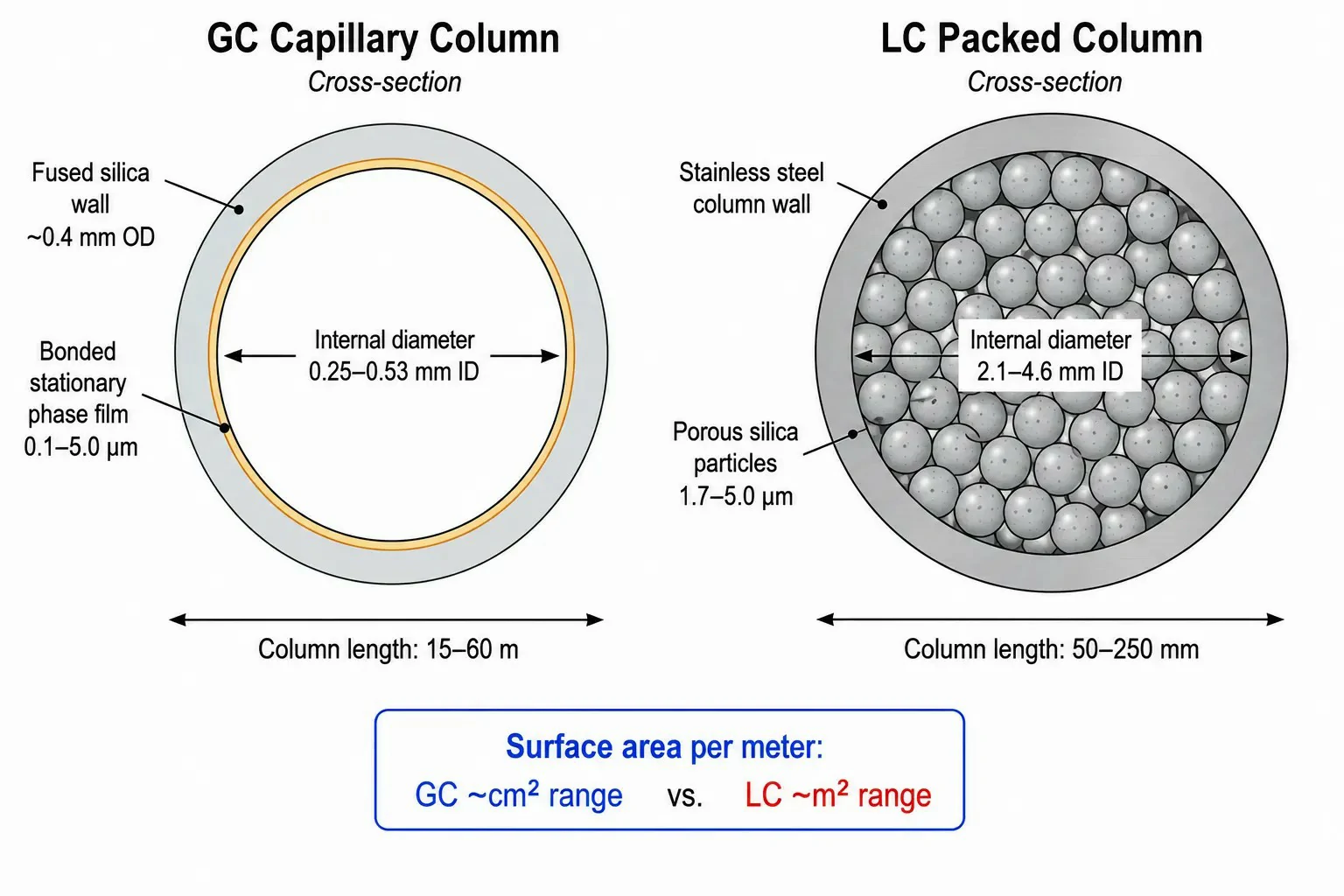 Figure 1: Comparative schematic of a GC capillary column cross-section (fused silica capillary wall with bonded stationary phase film) vs. an LC packed column cross-section (stainless steel tube with porous silica particles), with key dimensional parameters — column length, internal diameter, film thickness (GC) and particle size (LC) — annotated for each
The Separation Engine: Mobile Phase and Column Architecture
The fundamental distinction between GC and LC originates in the mobile phase state — a compressible gas in GC versus a nearly incompressible liquid in LC. This difference cascades through every aspect of column design, separation mechanism, and operational constraints.
Capillary Columns in GC: Length, Film Thickness, and Stationary Phase Selectivity
GC columns are open tubular capillaries, typically 15–60 m in length with internal diameters of 0.25–0.53 mm. The stationary phase is a thin film (0.1–5.0 μm) of liquid polymer bonded and cross-linked to the inner wall of the fused silica tubing. Separation occurs through partition between the mobile phase (carrier gas — helium, hydrogen, or nitrogen) and this stationary phase film, governed primarily by boiling point differences, with secondary contributions from polar interactions between the analyte and the stationary phase.
Stationary phase selectivity in GC follows a well-established polarity spectrum. Non-polar phases, such as 100% dimethylpolysiloxane, separate compounds primarily by boiling point. Mid-polarity phases, such as 5% phenyl-95% dimethylpolysiloxane, add π-π interaction capability for unsaturated compounds. Polar phases, such as polyethylene glycol (PEG/Wax), provide strong hydrogen-bonding interactions for alcohols, carboxylic acids, and aldehydes. The film thickness adds an independent dimension of selectivity: thin films (0.1–0.25 μm) reduce retention for high-boiling analytes and minimize column bleed at high temperatures, while thick films (1.0–5.0 μm) increase retention for highly volatile compounds that would otherwise elute with the solvent front. Selecting the appropriate phase and film thickness is the single most impactful decision in GC method development, analogous to choosing the bonded phase and particle size in LC.
Golay theory governs efficiency in capillary GC, where the minimum plate height (H_min) is inversely proportional to the square of the column internal diameter. Reducing the ID from 0.32 mm to 0.25 mm increases plate count per meter by approximately 60%, but also reduces sample capacity proportionally. This tradeoff between resolution and loading capacity mirrors the particle size tradeoff in LC: narrower capillaries provide superior separation efficiency at the cost of reduced sample mass tolerance.
Packed Columns in LC: Particle Morphology, Bonded Phase Chemistry, and Separation Modes
LC columns are short, packed-bed designs, typically 50–250 mm in length with internal diameters of 2.1–4.6 mm, filled with porous silica particles of 1.7–5 μm diameter. The stationary phase is a chemically bonded organic layer — most commonly octadecylsilane (C18) for reversed-phase separations — attached to the silica surface. Unlike GC, where the mobile phase plays a largely passive transport role, the LC mobile phase actively competes with the stationary phase for analyte interactions, making mobile phase composition the primary tuning variable in method development.
The bonded phase chemistry in LC determines the retention mechanism. C18 and C8 provide hydrophobic retention for non-polar to moderately polar compounds, covering approximately 80% of routine LC applications. HILIC (hydrophilic interaction liquid chromatography) retains polar compounds that show little or no retention on reversed-phase columns, making it essential for metabolites, carbohydrates, and polar natural products. Ion-exchange (IEX) and size-exclusion (SEC) columns address specific separation challenges — charged biomolecules and macromolecular mixtures, respectively — that fall outside the scope of both GC and reversed-phase LC. The ability to switch between these retention mechanisms on a single LC system, simply by changing the column and mobile phase, is a fundamental operational advantage over GC, which is largely restricted to volatility-based separations.
Recent advances in superficially porous particle (SPP) technology have narrowed the performance gap between LC and GC in terms of separation speed. A 2.6 μm SPP column operated at UHPLC pressures (15,000 psi) can achieve plate counts approaching 300,000 plates per meter — comparable to a 30 m × 0.25 mm GC capillary column operated under optimal linear velocity — but in minutes rather than tens of minutes. However, the fundamental difference in peak capacity distribution remains: GC distributes its resolving power over long retention time windows (30–60 min gradients common), while LC concentrates separation into shorter windows (5–30 min), making GC inherently better suited for very complex mixtures with hundreds of components.
Detection Systems: Information Content and Sensitivity
The choice between GC and LC is often determined not by the separation itself, but by what information the detector must provide. GC and LC detector technologies have evolved along fundamentally different paths, producing complementary rather than competing capabilities.
GC Detectors — From Universal to Element-Specific
The flame ionization detector (FID) remains the workhorse of GC detection, offering near-universal response to organic compounds with a linear dynamic range spanning seven orders of magnitude (10¹ to 10⁷ pg) and detection limits below 0.1 pg carbon per second. FID responds to any compound containing carbon-hydrogen bonds, producing a signal proportional to the number of carbon atoms reaching the detector flame, which simplifies quantitation because response factors for structurally similar compounds are often within 10–20% of each other. The FID does not respond to water, carbon dioxide, or inert carrier gases, making it ideal for trace analysis in aqueous matrices without the solvent interference that complicates LC-UV methods.
Selective detectors extend GC capability for specific analyte classes. The electron capture detector (ECD) achieves sub-picogram detection limits for halogenated, nitro, and conjugated carbonyl compounds, making it indispensable for environmental analysis of organochlorine pesticides and polychlorinated biphenyls — applications where LC-MS would require extensive sample cleanup and may not achieve comparable sensitivity. The nitrogen-phosphorus detector (NPD) provides selective response to nitrogen- and phosphorus-containing compounds at low picogram levels, used extensively in pharmaceutical and toxicological screening. The thermionic ionization mechanism in the NPD produces 10⁵–10⁶ times greater response for N/P compounds compared to hydrocarbons, enabling detection of nitrogen-containing drugs in complex biological extracts without chromatographic interference from the hydrocarbon matrix.
Mass spectrometry (MS) in GC is dominated by electron ionization (EI) at 70 eV, which produces highly reproducible fragmentation patterns that can be searched against commercial libraries such as the NIST Mass Spectral Library (containing spectra for approximately 350,000 compounds). This library-searchable fingerprint is unique to GC-MS: EI spectra are largely independent of instrument type and operating parameters, meaning a spectrum acquired on one GC-MS system can be matched against libraries built on entirely different instruments. Chemical ionization (CI), using reagent gases such as methane or ammonia, provides a softer alternative that preserves the molecular ion, useful for molecular weight confirmation when EI produces only weak or absent molecular ion signals.
LC Detectors — From Absorption to Universal Response
Ultraviolet-visible (UV/Vis) and photodiode array (PDA) detectors are the most widely used LC detectors, offering robust, cost-effective detection for compounds with chromophores. The PDA provides a spectral dimension — typically 190–800 nm — that aids peak identification and purity assessment, though the spectral information content is much lower than MS data. Sensitivity ranges from 0.1–1 ng on-column for strongly absorbing analytes (ε > 10⁵ L mol⁻¹ cm⁻¹) to 10–100 ng for weakly absorbing compounds. The fundamental limitation of UV detection in LC — its dependence on chromophore presence — is the mirror opposite of GC-FID, which responses universally to organic carbon regardless of structure.
Fluorescence detection (FLD) achieves 10–100 times higher sensitivity than UV for compounds with native fluorescence, reaching attomole detection limits for polycyclic aromatic hydrocarbons and aflatoxins. Evaporative light scattering detection (ELSD) and charged aerosol detection (CAD) provide near-universal response for non-volatile and semi-volatile analytes, bridging the gap for compounds lacking chromophores or fluorophores — carbohydrates, lipids, synthetic polymers, and pharmaceutical excipients — that are invisible to UV detection. However, ELSD and CAD produce non-linear response curves and shorter dynamic ranges compared to UV or MS, complicating quantitation across wide concentration ranges.
LC-MS interfaces use atmospheric pressure ionization (API) techniques — electrospray ionization (ESI), atmospheric pressure chemical ionization (APCI), and atmospheric pressure photoionization (APPI) — which generate ions at atmospheric pressure before mass analysis. Unlike the hard ionization in GC-EI, API techniques are soft, producing primarily molecular ions ([M+H]⁺, [M-H]⁻, or adducts) with minimal fragmentation. The practical consequence is substantial: LC-MS spectra cannot be matched against standardized libraries in the same way as EI spectra. Identification in LC-MS relies on accurate mass measurement (typically within 3–5 ppm on a Q-TOF or Orbitrap), retention time matching against authentic standards, and MS/MS fragmentation patterns interpreted manually or matched against in-house or community-curated libraries (e.g., mzCloud, MassBank). This difference in identification confidence — library-searchable EI spectra versus accurate-mass- and retention-time-dependent LC-MS identification — is one of the most important practical distinctions between GC and LC for non-targeted analysis.
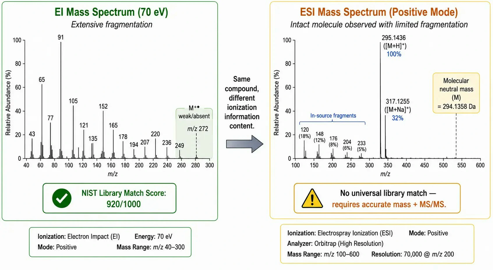 Figure 2: Side-by-side mass spectral comparison: EI spectrum (70 eV) of a model compound with annotated library-matched fragment ions versus ESI spectrum of the same compound showing [M+H]⁺, sodium adduct [M+Na]⁺, and in-source fragments, with confidence assignment levels and library match scores annotated
The GC-MS vs. LC-MS Gap: Why EI Spectra Are Searchable
The library-searchable nature of EI spectra makes GC-MS the preferred platform for non-targeted screening of unknown compounds in environmental, forensic, and metabolomics applications. When a GC-MS analysis of an environmental water extract detects an unknown peak at retention time 12.3 min, the EI spectrum is acquired, background-subtracted, and searched against the NIST library, often producing a correct identification within minutes. The same unknown analyzed by LC-MS would require interpretation of the accurate mass, isotopic pattern, and MS/MS fragmentation — a process that may take hours and still yield an identification with lower confidence, particularly if the compound is not represented in a curated LC-MS library.
However, this library-searchability comes at a cost: EI fragments molecules so extensively that the molecular ion is often absent or very weak, making molecular weight determination uncertain without parallel CI analysis. LC-MS preserves the molecular ion, providing unambiguous molecular weight information that is essential for structural characterization. The two techniques are therefore complementary: GC-MS for rapid, library-based identification of volatile and semi-volatile unknowns; LC-MS for targeted quantitation and structural characterization of polar, non-volatile compounds where molecular weight information is critical.
Quantitation Strategies: Accuracy, Reproducibility, and Matrix Effects
The quantitation paradigms in GC and LC differ in ways that directly affect method development time, validation burden, and data quality — factors that become decisive in regulated environments such as pharmaceutical quality control and clinical research.
GC offers inherent advantages in quantitation reproducibility. Retention time precision in temperature-programmed GC is typically better than 0.05% relative standard deviation (RSD) across an analytical batch, compared to 0.5–2% RSD in gradient LC. This stability originates from the simpler and more reproducible fluidic environment: gas flow at moderate pressures produces negligible frictional heating, and the absence of solvent mixing gradients eliminates the retention time variability caused by gradient dwell volume differences between LC systems. For laboratories performing multi-batch quantitation across instruments, GC retention time stability simplifies peak tracking and automated data processing, reducing the data review burden.
More importantly, matrix effects in GC with FID or EI-MS are generally modest compared to LC-ESI-MS. The universal FID response — where signal is proportional to carbon mass — is largely unaffected by co-eluting matrix components, provided they do not overwhelm the detector dynamic range. EI-MS is subject to matrix-induced signal suppression or enhancement in the ion source, but the effect is typically 10–30% for most sample types, compared to the 50–500% matrix effects commonly observed in LC-ESI-MS. This means that GC quantitation methods can often use simple internal standards (e.g., a structurally similar hydrocarbon or a single deuterated analog) without requiring isotopically labeled internal standards for every analyte.
LC-ESI-MS quantitation, by contrast, is heavily affected by matrix effects arising from the competition between analyte and co-eluting matrix components for ionization in the electrospray droplet. Ion suppression — where matrix components interfere with droplet formation, desolvation, or ion evaporation — can reduce analyte signal by orders of magnitude, and the effect varies between samples, injection-to-injection within a batch, and across the gradient profile. For accurate quantitation in complex biological matrixes (plasma, urine, tissue extracts), stable isotope-labeled internal standards (SIL-IS) for each analyte are considered essential in regulated bioanalysis, as only an internal standard eluting at the same retention time can compensate for matrix-induced signal variability. The synthesis or purchase of SIL-IS represents a significant cost and timeline factor: a single ²H- or ¹³C-labeled internal standard may cost $500–$5,000 and require 4–8 weeks lead time. For methods quantifying 10–50 analytes simultaneously, the SIL-IS budget alone can reach $50,000 or more, a cost entirely absent from GC-FID methods and substantially lower in GC-MS methods using non-isotopic internal standards.
Targeted metabolomics services routinely employ both GC-MS and LC-MS/MS platforms, selecting the quantitation strategy based on analyte polarity, matrix complexity, and required throughput.
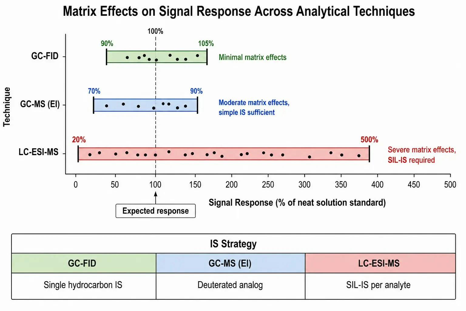 Figure 3: Side-by-side comparison chart of matrix effect magnitude — GC-FID, GC-MS (EI), and LC-ESI-MS — with typical signal response ranges for spiked analytes in a biological matrix, annotated with recommended internal standard strategies for each combination
Sample Preparation and Derivatization: The Hidden Workflow Cost
Sample preparation represents a significant and often underestimated cost in both GC and LC workflows, but the nature of that cost differs fundamentally between the two techniques.
GC sample preparation is dominated by the requirement for volatile, thermally stable analytes. Non-volatile or thermally labile compounds must be chemically derivatized to increase volatility and reduce thermal degradation. The most common derivatization strategy is silylation — replacing active hydrogens in -OH, -NH, -SH, and -COOH groups with trimethylsilyl (TMS) groups using reagents such as BSTFA (N,O-bis(trimethylsilyl)trifluoroacetamide) or MSTFA. A typical derivatization protocol adds 30–60 minutes to sample preparation time and introduces variables — reagent purity, reaction temperature and duration, moisture exclusion, and byproduct formation — that affect reproducibility. For multi-analyte methods targeting compounds with different functional groups, no single derivatization condition is optimal for all analytes, requiring compromise conditions that may sacrifice sensitivity for some compounds.
Beyond derivatization, GC sample preparation includes liquid-liquid extraction (LLE), solid-phase extraction (SPE), headspace (HS) sampling, and solid-phase microextraction (SPME) for volatile and semi-volatile analytes from complex matrices. The key practical advantage of HS and SPME is that they introduce only volatile analytes into the GC system, leaving non-volatile matrix components behind — effectively providing on-column matrix elimination that LC cannot achieve without extensive off-line cleanup. Laboratories running routine GC methods for volatile organic compounds (VOCs) in environmental water can process 50–100 samples per day without column degradation precisely because the non-volatile matrix (humic acids, salts, biological debris) never reaches the column.
LC sample preparation offers broader flexibility. Protein precipitation (PPT), SPE, and dilute-and-shoot workflows are compatible with all sample types — aqueous, organic, biological fluid — because LC systems are designed to handle liquid injections. The absence of a volatilization requirement means that polar metabolites, peptides, and proteins can be analyzed with minimal sample manipulation. However, the lack of a "volatility gate" means that everything injected — including non-volatile matrix components — enters the column, contributing to column contamination, backpressure buildup, and gradual performance degradation. A typical biological LC-MS sequence of 100 injections without adequate SPE cleanup may require column replacement or intensive washing, whereas a GC-MS sequence analyzing headspace extracts of the same samples may operate for thousands of injections between column trims.
The practical cost comparison is scenario-dependent. A GC method requiring derivatization for each of 500 samples adds approximately 250–500 hours of technician time per campaign — a cost that may exceed the entire consumables budget for an equivalent LC-MS method. Conversely, an LC-MS method processing 1,000 crude plasma extracts that requires column replacement after every 300 injections adds $500–$1,000 per 1,000 samples in column costs, compared to a GC headspace method analyzing 1,000 water samples with negligible column cost. The selection of sample preparation strategy is therefore inseparable from the platform decision: the apparent cost advantage of one technique may be reversed when sample preparation costs are fully accounted.
 Figure 4: Workflow cascade comparing GC sample preparation (LLE/SPE/HS/derivatization) vs. LC sample preparation (PPT/SPE/dilute-and-shoot) with typical processing times and key bottlenecks annotated for each parallel workflow
Method Development: A Practical Comparison
The method development workflow for GC and LC differs in the number of tunable parameters, optimization strategies, and typical timelines — factors that directly affect laboratory productivity and time-to-data.
GC method development centers on temperature program optimization. The primary variables are: initial temperature (typically 40–80°C), ramp rate (5–20°C/min), final temperature (250–325°C, limited by column thermal stability), and hold times at initial and final temperatures. Isothermal separations, useful for simple mixtures with a narrow boiling range, are optimized by selecting a single temperature that balances resolution and run time. Multi-ramp temperature programs, required for samples with a wide boiling point distribution (e.g., petroleum hydrocarbons, essential oils), add complexity but follow established optimization heuristics: start with a slow ramp (5°C/min) for complex mixtures, increase the ramp rate when faster throughput is needed, and adjust the final hold time to ensure complete elution of high-boiling compounds to avoid carryover. A skilled chromatographer can typically develop and validate a GC-FID method for a well-characterized analyte in 1–2 days, with temperature program optimization requiring 5–10 trial runs.
LC method development is inherently more multidimensional. The tunable parameters include stationary phase chemistry (C18, C8, phenyl, HILIC, IEX, mixed-mode), mobile phase composition (organic modifier type and percentage, pH, buffer concentration, ion-pairing reagent), gradient profile (steepness, initial and final composition, column volumes), column temperature (20–60°C), and flow rate. The interdependence of these parameters makes univariate optimization impractical for complex separations. Modern LC method development increasingly employs automated column and solvent screening systems that test 8–24 phase-gradient combinations in a single unattended sequence, followed by design-of-experiment (DoE) optimization of the most promising conditions. A typical LC method development timeline is 2–5 days, with the screening phase consuming 1–2 days and the optimization and robustness testing requiring an additional 1–3 days.
An important practical distinction is that LC methods can be developed and optimized for multiple detection modes (UV at multiple wavelengths, MS with different ionization parameters) within the same development cycle, whereas GC method development is typically coupled to a single detector choice (FID, ECD, or MS) from the outset. The decision to use GC-MS rather than GC-FID, for example, changes the method development timeline because MS requires different sample capacity optimization (avoiding detector saturation from high-concentration analytes) and additional ion source temperature optimization. LC-MS method development additionally requires optimization of ESI or APCI parameters — sheath gas flow, capillary temperature, spray voltage — that affect ionization efficiency independently of the chromatographic separation, adding approximately 0.5–1 day to the development timeline.
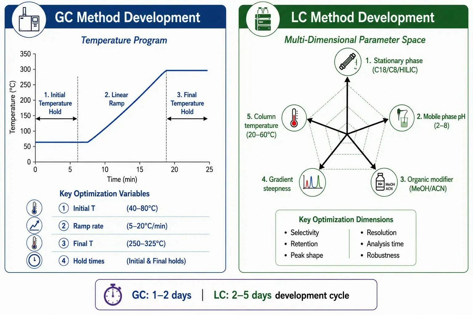 Figure 5: Parameter comparison infographic showing GC temperature program variables (initial T, ramp rate, final T, hold time) vs. LC method development variables (column chemistry, mobile phase pH, organic modifier, gradient steepness, temperature), with typical optimization timelines annotated for each pathway
Operational Costs and Laboratory Infrastructure
The total cost of ownership for GC and LC platforms diverges along three axes: consumables, infrastructure, and maintenance. These costs accumulate over the instrument lifetime (typically 7–10 years) and can equal or exceed the initial capital investment.
GC operational costs are dominated by carrier gas and consumables. Helium, the most common GC carrier gas, has experienced price increases of 200–300% over the past decade due to global supply constraints, with a 49-liter cylinder now costing $300–$600 depending on purity and location. Hydrogen, generated electrolytically from water using a hydrogen generator (capital cost $3,000–$8,000), provides comparable or superior separation efficiency at a fraction of the per-analysis carrier gas cost, though safety considerations (hydrogen flammability) require proper ventilation and leak detection. GC consumables — injection septa ($1–$3 each, replaced every 50–100 injections), liner ($5–$15 each, replaced every 50–200 injections depending on sample cleanliness), and ferrule sets ($5–$10 per column installation) — are relatively inexpensive. The column itself ($300–$700) may last 500–2,000 injections depending on sample matrix, with regular trimming of 5–10 cm from the column inlet to restore performance after 50–200 injections. There are no solvent purchase or disposal costs for GC-FID analysis, though GC-MS requires a vacuum system (turbomolecular pump, backing pump) with annual maintenance costs of $500–$2,000.
LC operational costs are dominated by solvents, columns, and high-pressure system maintenance. HPLC-grade acetonitrile ($80–$150 per liter) and methanol ($40–$80 per liter) are consumed at rates of 0.5–2 L per day for routine LC-MS operation, representing an annual solvent cost of $10,000–$40,000 for a single instrument running continuously. Solvent disposal adds $0.50–$2.00 per liter of mixed organic-aqueous waste. LC columns for UHPLC ($400–$900 each) typically last 500–2,000 injections, with guard columns ($50–$150 each, replaced every 100–500 injections) protecting the analytical column lifetime. High-pressure pump seals in UHPLC systems require replacement every 6–12 months ($200–$500 in parts and labor), and the detector flow cell or ESI spray chamber may require periodic cleaning or replacement ($500–$3,000). The total annual consumables and maintenance cost for a continuously operated UHPLC-MS system typically ranges from $15,000–$50,000, compared to $3,000–$10,000 for a GC-MS system operated at equivalent throughput.
These cost differences are partially offset by the higher sample throughput of LC methods (typically 5–15 minute run times vs. 20–45 minutes for GC) and the broader analyte coverage that may eliminate the need for a second orthogonal technique. A laboratory analyzing both polar and non-polar analytes may require only LC-MS; a laboratory relying solely on GC-MS for the same analyte scope would require derivatization for non-volatile compounds, adding significant per-sample cost.
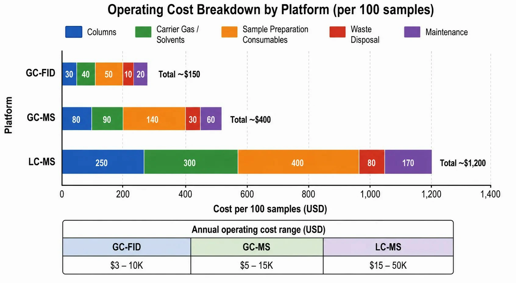 Figure 6: Bar chart comparing estimated per-100-sample cost breakdown for GC-FID, GC-MS, and LC-MS platforms, segmented by columns, carrier gas/solvents, sample preparation, consumables, and waste disposal, with total cost per sample annotated
Decision Framework: Which Technique for Which Analytical Objective
The optimal platform choice depends on matching instrument capability to analytical objectives across three broad scenarios.
Choose GC when the analytical objective involves volatile and thermally stable compounds (boiling point < 350°C, molecular weight typically < 500 Da), particularly when non-targeted identification is required. GC-MS with EI provides library-searchable mass spectra that enable rapid identification of unknowns in environmental contaminants, food aroma compounds, petrochemical products, and forensic toxicology specimens. GC-FID is the preferred platform for routine quantitation of hydrocarbon-based analytes in relatively clean matrices — residual solvents in pharmaceuticals, fatty acid methyl esters in food, volatile organic compounds in water — where the universal carbon response simplifies quantitation without the need for matrix-matched calibration. Laboratories operating under solvent usage restrictions or with limited access to LC-MS instrumentation will also find GC a cost-effective alternative for suitable analytes.
Choose LC when the analyte population includes polar, thermally labile, or high-molecular-weight compounds (> 500 Da). LC-MS with ESI provides the sensitivity and selectivity required for pharmaceutical bioanalysis, proteomics, lipidomics, and the analysis of polar metabolites that are not amenable to GC even after derivatization. The ability to switch between reversed-phase, HILIC, and ion-exchange separations on the same LC system provides flexibility for multi-class analyte panels — for example, combining hydrophobic drugs, polar metabolites, and charged amino acids in a single analytical sequence. LC-UV/FLD methods are well-suited for quality control applications where the analytes have adequate chromophores or native fluorescence and where the lower instrument cost and operational simplicity outweigh the need for universal detection.
Use both GC and LC when the analytical scope spans compound classes with divergent physicochemical properties. Non-targeted metabolomics is the canonical example: a combined GC-MS (for volatile organic acids, sugars, and derivatized polar metabolites) and LC-MS (for non-volatile lipids, amino acids, and polar conjugates) workflow covers 70–90% of the detectable metabolome, whereas either technique alone covers 30–50%. Similarly, comprehensive food safety analysis combines GC for volatile contaminants (pesticides, PCBs, processing contaminants) and LC for non-volatile hazards (mycotoxins, veterinary drug residues, food additives). Metabolomics analysis services leverage both GC-MS and LC-MS platforms to provide comprehensive metabolic coverage across diverse sample types.
For laboratories with limited instrumentation budgets, the practical recommendation is to invest in LC-MS first if the primary workload involves biological or pharmaceutical samples, and GC-MS first if the primary workload involves environmental, petrochemical, or volatile organic analysis. A dual-platform laboratory provides the most robust analytical capability and the flexibility to handle virtually any sample type encountered in a modern analytical laboratory.
Conclusion
GC and LC are not competing technologies in the sense that one is universally superior — they are complementary separation platforms optimized for different regions of chemical space. GC delivers unparalleled separation efficiency for volatile and semi-volatile compounds, combined with the unique advantage of library-searchable EI mass spectra for non-targeted identification and robust quantitation with minimal matrix effects. LC provides flexible separation modes that accommodate the full range of polar to non-polar, volatile to non-volatile compounds, with detection systems (particularly ESI-MS) that offer exceptional sensitivity for biological molecules but demand more rigorous quantitation strategies to manage matrix effects. The decision between them, and the decision to invest in both, should be guided by a systematic assessment of the analyte population, the required identification confidence, the quantitation accuracy demands, and the operational budget — not by assumptions about which technique is "better." Laboratories that understand these tradeoffs can allocate instrumentation resources strategically, matching platform capability to analytical need rather than defaulting to a single technique.
Frequently Asked Questions
Can GC and LC use the same type of detector?
No. GC detectors operate at high temperature and atmospheric or reduced pressure, designed for gas-phase analytes. LC detectors operate at ambient temperature and pressure in the liquid phase. The only detector type that bridges both techniques is mass spectrometry, but the ionization methods are entirely different — EI in GC-MS versus ESI/APCI in LC-MS — making the mass spectrometers themselves different instruments optimized for each ionization environment.
Why is GC considered more reproducible than LC for retention times?
GC retention time reproducibility benefits from three factors: temperature programming provides a highly reproducible thermal environment, gas flow at moderate pressure generates negligible frictional heating, and the single-component mobile phase eliminates the gradient mixing and dwell volume variability inherent in LC. Retention time RSD in GC is typically less than 0.1%, compared to 0.5–2% in LC.
Do I always need derivatization for GC analysis?
Only if your analytes are non-volatile or thermally labile. Many compounds — hydrocarbons, solvents, essential oil components, fatty acid methyl esters, halogenated pesticides — are directly amenable to GC without derivatization. Derivatization is required when the compound contains polar functional groups (-OH, -COOH, -NH₂) that cause strong intermolecular interactions and reduce volatility. More than 50% of published GC methods for biological samples involve some form of derivatization.
Can LC-MS replace GC-MS for non-targeted screening?
For volatile and semi-volatile compounds, no. EI mass spectra are library-searchable against comprehensive databases (NIST, Wiley) that contain 350,000+ compounds with instrument-independent fragmentation patterns. LC-MS identification relies on accurate mass, retention time matching, and MS/MS interpretation — a slower and less definitive process for unknown identification. LC-MS can replace GC-MS for targeted quantitation of known analytes, but for true non-targeted screening, the two techniques remain complementary.
Which technique has lower cost per sample?
For volatile analytes in clean matrices (headspace GC-MS for VOCs in water): GC. The per-sample consumable cost is negligible, and throughput is high. For polar analytes in biological matrices (LC-MS for drugs in plasma): LC may be more cost-effective because derivatization-free analysis avoids 250–500 hours of technician time per campaign, despite higher solvent and column costs. For derivatization-required GC methods, LC is almost always more cost-effective per sample.
What samples cannot be analyzed by GC at all?
Inorganic salts, most proteins and peptides, nucleic acids, highly polar ionic compounds (unless derivatized), thermally unstable analytes that degrade below 150°C, and compounds with molecular weights above approximately 1,000 Da (limited by volatility) cannot be analyzed by GC without derivatization. Many of these are routine samples for LC-MS analysis.
How do I choose between GC-MS and LC-MS for metabolomics?
Use GC-MS for primary metabolites — organic acids, sugars, amino acids (as derivatives), fatty acids — and volatile secondary metabolites. Use LC-MS for lipids, polar conjugates, and secondary metabolites that fall outside the GC-amenable volatile range. For comprehensive metabolome coverage, use both: GC-MS and LC-MS datasets are complementary, each identifying compounds invisible to the other technique, together covering 70–90% of the detectable metabolome.
References
- Grob RL, Barry EF. Modern Practice of Gas Chromatography. 4th ed. Hoboken: Wiley-Interscience; 2004. 10.1002/0471651141
- Neue UD. HPLC Columns: Theory, Technology, and Practice. New York: Wiley-VCH; 1997. 10.1002/9780471988860
- Gates SC, Sweeley CC. Quantitative metabolic profiling based on gas chromatography. Clinical Chemistry. 1978;24(10):1663-1673. 10.1093/clinchem/24.10.1663
- Zhao YY, Cheng XL. Metabolomics: Methods and Protocols. Methods in Molecular Biology. 2021;2276:1-15. 10.1007/978-1-0716-1266-8_1
- Harris DC. Quantitative Chemical Analysis. 9th ed. New York: W.H. Freeman; 2015. ISBN: 978-1464135385.
- Moco S, Bino RJ, Vorst O, et al. A liquid chromatography-mass spectrometry-based metabolome database for tomato. Plant Physiology. 2006;141(4):1205-1218. 10.1104/pp.106.078428
- Kataoka H, Lord HL, Pawliszyn J. Applications of solid-phase microextraction in food analysis. Journal of Chromatography A. 2000;880(1-2):35-62. 10.1016/S0021-9673(00)00309-5
- Niessen WMA. Liquid Chromatography-Mass Spectrometry. 3rd ed. Boca Raton: CRC Press; 2006. 10.1201/9781420014549
- Matuszewski BK, Constanzer ML, Chavez-Eng CM. Strategies for matrix effect assessment in quantitative LC-MS/MS. Analytical Chemistry. 2003;75(13):3019-3030. 10.1021/ac020361s
- Fiehn O. Metabolomics by gas chromatography-mass spectrometry. Current Protocols in Molecular Biology. 2016;114:30.4.1-30.4.32. 10.1002/0471142727.mb3004s114