- Service Details
- Demo
- FAQ
- Publications
What is Principal Component Analysis?
Principal Component Analysis (PCA) is a statistical technique used for dimensionality reduction. It transforms a large set of variables into a smaller one that still contains most of the information in the large set. This transformation is achieved through the identification of principal components, which are new variables constructed as linear combinations of the original variables.
PCA works by finding the directions (principal components) along which the variation in the data is maximized. The first principal component captures the largest amount of variation, the second principal component captures the next largest amount, and so on. These principal components are orthogonal to each other, ensuring that there is no redundancy in the information they carry.
Key Steps in PCA
- Standardization: The data is scaled to have a mean of zero and a variance of one.
- Covariance Matrix Computation: The covariance matrix of the data is calculated to understand how the variables are correlated with each other.
- Eigenvalue and Eigenvector Calculation: Eigenvalues and eigenvectors of the covariance matrix are computed. The eigenvectors determine the directions of the new feature space, and the eigenvalues determine their magnitude.
- Principal Components Formation: The eigenvectors with the largest eigenvalues form the principal components.
- Data Projection: The original data is projected onto the new feature space defined by the principal components.
Why is Principal Component Analysis Needed?
Dimensionality Reduction
Biological datasets, such as those generated from high-throughput sequencing or mass spectrometry, often contain a large number of variables. Handling such high-dimensional data can be challenging due to the "curse of dimensionality." PCA reduces the dimensionality of the data, making it more manageable while retaining most of the original information.
Noise Reduction
High-dimensional data can be noisy, which can obscure meaningful patterns. PCA helps in filtering out the noise by focusing on the components that capture the most variance in the data.
Data Visualization
PCA simplifies the visualization of complex data. By reducing the data to two or three principal components, it becomes easier to visualize and interpret the underlying patterns and relationships in the data.
Feature Extraction
PCA helps in identifying the most significant features in the data, which can be useful for further analysis and model building.
Multicollinearity Elimination
In datasets where variables are highly correlated, PCA can help in transforming the correlated variables into a set of uncorrelated principal components, thus addressing multicollinearity issues.
What We Can Provided?
At Creative Proteomics, PCA is an integral part of our data analysis toolkit. We leverage PCA to enhance the interpretation and understanding of complex biological data, ensuring that our clients receive accurate and insightful results.
PCA in Proteomics
In proteomics, PCA is invaluable for analyzing large datasets generated from mass spectrometry and other proteomic technologies. Proteomic datasets often contain thousands of variables representing different proteins or peptides. PCA helps in identifying the most significant variables and understanding their relationships, enabling the discovery of key biomarkers and the elucidation of underlying biological processes.
Key Applications in Proteomics:
- Biomarker Discovery: PCA helps in identifying proteins that are differentially expressed between different sample groups, such as healthy vs. diseased.
- Protein Expression Profiling: By reducing the dimensionality of the data, PCA enables the visualization of protein expression patterns, facilitating the understanding of biological functions and pathways.
- Comparative Analysis: PCA allows for the comparison of protein expression profiles under different experimental conditions, aiding in the identification of treatment effects or disease mechanisms.
PCA in Metabolomics
In metabolomics, PCA is used to analyze complex datasets generated from techniques like nuclear magnetic resonance (NMR) spectroscopy and mass spectrometry. Metabolomic datasets contain a wide range of metabolites with varying concentrations, making PCA a crucial tool for reducing complexity and highlighting significant metabolic changes.
Key Applications in Metabolomics:
- Metabolic Profiling: PCA enables the identification of key metabolites that differentiate between sample groups, such as different stages of disease or responses to treatment.
- Pathway Analysis: By highlighting the most significant changes in metabolite levels, PCA aids in understanding the metabolic pathways involved in different biological processes.
- Sample Classification: PCA helps in classifying samples based on their metabolic profiles, which is useful for disease diagnosis and prognosis.
PCA in Glycomics
Glycomics, the study of glycans (sugar molecules) and their roles in biological systems, generates highly complex datasets due to the structural diversity of glycans. PCA is particularly useful in glycomics for simplifying these complex datasets and extracting meaningful patterns.
Key Applications in Glycomics:
- Glycan Structure Analysis: PCA assists in identifying and characterizing different glycan structures, which is crucial for understanding their biological functions and roles in disease.
- Comparative Glycomics: By reducing the dimensionality of glycan datasets, PCA facilitates the comparison of glycan profiles between different sample groups, such as cancerous vs. non-cancerous tissues.
- Biomarker Identification: PCA helps in discovering glycan biomarkers that can be used for disease diagnosis, prognosis, and monitoring therapeutic responses.
Workflow of PCA at Creative Proteomics
Data Collection: We start by collecting high-quality data from our clients using state-of-the-art instruments and methodologies. This includes sample preparation, instrument calibration, and data acquisition protocols tailored to each specific project.
Data Preprocessing: The collected data undergoes rigorous preprocessing to remove technical variability and standardize values. This step involves data normalization, scaling, and transformation to ensure that the PCA results are robust and reliable.
PCA Implementation: Using advanced statistical software and algorithms, we implement PCA to transform the high-dimensional data into a set of principal components. This process involves calculating the covariance matrix, extracting eigenvalues and eigenvectors, and forming the principal components that capture the most variance in the data.
Result Interpretation: The principal components are analyzed to identify significant patterns and trends within the data. Our experts interpret these components to provide insights into the biological relevance of the identified patterns. This includes identifying clusters of similar samples, outliers, and potential biomarkers.
Detailed Reporting and Visualization: We provide comprehensive reports and visualizations to our clients. These reports include detailed descriptions of the PCA process, interpretation of the principal components, and visualizations such as score plots and loading plots that make it easy to understand the data's structure and key findings.

The horizontal coordinate is the test sample and the vertical coordinate corresponds to the PC1 value of the sample in the PCA analysis

PCA plot of quality control samples

Two-dimensional graph of PCA analysis of grouped samples

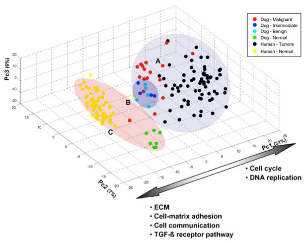
Three-dimensional graph of PCA analysis of grouped samples
What does PC1 and PC2 mean?
In Principal Component Analysis (PCA), PC1 (Principal Component 1) and PC2 (Principal Component 2) refer to the first and second principal components, respectively. These components are new axes in the transformed space that capture the maximum variance in the data.
- PC1: The first principal component is the direction that captures the largest amount of variance in the data. It is the most important component because it explains the most significant variation within the dataset.
- PC2: The second principal component is orthogonal (perpendicular) to PC1 and captures the second largest amount of variance. It represents the second most important pattern in the data.
The principal components are linear combinations of the original variables and are ordered by the amount of variance they capture, with PC1 capturing the most variance, followed by PC2, and so on.
How do you interpret the results of PCA?
Interpreting the results of PCA involves several steps:
1. Variance Explained: Look at the proportion of total variance explained by each principal component. This is usually visualized in a scree plot.
2. Loadings: Examine the loadings of the original variables on each principal component. High absolute values indicate that the variable significantly contributes to that principal component.
3. Scores: Analyze the scores, which are the projections of the original data onto the principal components. This helps to identify patterns, clusters, or outliers in the data.
4. Biplot: A biplot can be used to visualize both the scores and the loadings on the same plot. This provides insights into the relationships between the variables and the observations.
5. Interpret Principal Components: Understand what each principal component represents in terms of the original variables. This involves interpreting the direction and magnitude of the loadings.
What tools and software are commonly used for PCA?
Several tools and software packages are commonly used for PCA, including:
- R: Packages like prcomp, princomp, and FactoMineR are popular for performing PCA.
- Python: Libraries such as scikit-learn (with PCA module), numpy, and pandas are frequently used for PCA.
- MATLAB: Functions like pca are available for conducting PCA in MATLAB.
- SPSS: A statistical software package that offers PCA under its dimension reduction options.
- SAS: Includes procedures like PROC PRINCOMP for performing PCA.
- JMP: Provides an intuitive interface for PCA and other multivariate techniques.
How can PCA be integrated with other analytical techniques?
PCA can be integrated with other analytical techniques in several ways:
1. Cluster Analysis: Use PCA to reduce the dimensionality of the data before applying clustering algorithms like K-means or hierarchical clustering. This helps to improve the clustering performance by removing noise and redundant features.
2. Regression Analysis: PCA can be used to handle multicollinearity in regression models. Principal components can be used as predictors instead of the original correlated variables.
3. Machine Learning: PCA is often used as a preprocessing step in machine learning workflows to reduce the dimensionality of the feature space, which can lead to improved model performance and reduced computational cost.
4. Visualization: PCA is used to transform high-dimensional data into two or three principal components for easier visualization and interpretation.
5. Feature Selection: By identifying the most important principal components, PCA can help in selecting the most relevant features for further analysis.
What is the difference between PCA and other dimensionality reduction techniques?
PCA is one of several dimensionality reduction techniques. Here's how it compares to others:
- PCA vs. Linear Discriminant Analysis (LDA): PCA is an unsupervised method that focuses on maximizing variance, whereas LDA is a supervised method that maximizes the separation between predefined classes.
- PCA vs. Independent Component Analysis (ICA): PCA finds components that maximize variance and assumes components are orthogonal, while ICA finds statistically independent components, often used for blind source separation.
- PCA vs. t-Distributed Stochastic Neighbor Embedding (t-SNE): PCA is a linear technique, while t-SNE is a non-linear technique designed for visualizing high-dimensional data by preserving local structures.
- PCA vs. Factor Analysis: PCA focuses on variance and uses orthogonal components, while factor analysis models the data using latent factors and accounts for the underlying structure.
- PCA vs. Autoencoders: Autoencoders are a non-linear technique based on neural networks, capable of capturing complex patterns, whereas PCA is limited to linear transformations.
How does PCA handle missing data in datasets?
PCA requires complete datasets without missing values. There are several ways to handle missing data before applying PCA:
Imputation: Replace missing values with estimated values using methods such as mean imputation, median imputation, or more sophisticated techniques like k-nearest neighbors (KNN) imputation.
Deletion: Remove any rows or columns with missing values, though this can lead to loss of valuable information.
Expectation-Maximization (EM): An iterative method that estimates missing values and updates PCA results until convergence.
Multiple Imputation: Generate several different plausible datasets by filling in missing values and perform PCA on each, then combine the results.
Can PCA be applied to time-series data?
Yes, PCA can be applied to time-series data. There are several ways to approach this:
Static PCA: Treat time points as separate variables and apply PCA to the entire dataset to identify overall patterns.
Dynamic PCA: Apply PCA to time-series data in a rolling or sliding window manner to capture temporal dynamics.
Multivariate Time-Series: Combine multiple time-series into a multivariate dataset and apply PCA to analyze the relationships between them.
What is the role of eigenvalues and eigenvectors in PCA?
Eigenvalues and eigenvectors play a crucial role in PCA:
- Eigenvalues: Represent the amount of variance captured by each principal component. The eigenvalues are used to rank the principal components.
- Eigenvectors: Define the directions of the principal components. Each eigenvector is a linear combination of the original variables and indicates how much each variable contributes to the principal component.
The principal components are the eigenvectors of the covariance matrix of the original data, and the eigenvalues indicate the significance of these components.
How many principal components should be retained in an analysis?
The number of principal components to retain depends on the variance explained and the specific application. Common criteria include:
- Variance Explained: Retain enough components to explain a high percentage of the total variance (e.g., 90-95%).
- Scree Plot: Identify the "elbow" point in a scree plot where the explained variance starts to level off.
- Kaiser Criterion: Retain components with eigenvalues greater than 1.
- Cumulative Proportion: Consider the cumulative proportion of variance explained by the retained components.
What is the significance of the scree plot in PCA?
The scree plot is a visual tool used in PCA to determine the number of principal components to retain. It plots the eigenvalues in descending order against the principal component number. The key features of the scree plot are:
- Elbow Point: The point where the plot starts to flatten out, indicating diminishing returns in terms of variance explained by additional components.
- Variance Explained: Helps to visualize how much variance each component captures and aids in deciding the number of components to retain.
How does PCA help in data visualization?
PCA helps in data visualization by reducing high-dimensional data to two or three dimensions, which can be plotted easily. This provides a clear and interpretable representation of the data, highlighting:
- Patterns and Trends: Revealing the main patterns and trends in the data.
- Clusters: Identifying clusters or groupings of similar observations.
- Outliers: Detecting outliers that deviate significantly from the rest of the data.
Common visualizations include score plots, loading plots, and biplots, which combine both scores and loadings to show relationships between variables and observations.
NUDT22 promotes cancer growth through pyrimidine salvage and the TCA cycle
Melanie Walter, Florian Mayr, Bishoy Magdy Fekry Hanna, et al
Journal: Research Square
Year: 2022
https://doi.org/10.21203/rs.3.rs-1491465/v1
Transcriptomics, metabolomics and lipidomics of chronically injured alveolar epithelial cells reveals similar features of IPF lung epithelium
Willy Roque, Karina Cuevas-Mora, Dominic Sales, Wei Vivian Li, Ivan O. Rosas, Freddy Romero
Journal: bioRxiv
Year: 2020
https://doi.org/10.1101/2020.05.08.084459