Meta Intent: A physics-driven, high-readability guide to designing and optimizing sucrose-based rate-zonal centrifugation for high-resolution separation of macromolecular particles.
Rate-zonal centrifugation is often presented as a simple workflow. Load the sample onto a preformed gradient. Spin for a defined time. Collect the bands before they pellet. That summary is not wrong. It is simply too thin to explain why one run gives crisp fractions and the next gives a blurred column.
The real method lives in the details that ordinary protocol pages compress into a few lines. A particle does not move through a gradient at one fixed speed. It slows as the medium changes beneath it. It does not behave like a perfect sphere unless it actually is one. And a separation is not protected just because the rotor reached the target speed. Resolution can be damaged at loading, during sedimentation, and again when the rotor stops.
That is why rate-zonal centrifugation is best understood as a transport problem in a rotating field. Once the problem is framed that way, the optimization logic becomes much clearer. The design question is no longer "Which sucrose range is commonly used?" The better question is "How will this specific particle class move through this specific gradient, at this temperature, in this rotor, under this braking policy?"
That shift matters most when the sample is heterogeneous. Exosomes are not identical spheres. Ribosomes do not all carry the same mass distribution or assembly state. Viral capsids can be empty, full, partially full, or aggregated. Those differences change motion in ways that are easy to miss if the method is treated as a recipe instead of a physical system. A gradient that looks reasonable on paper can still fail because the sample entered too deeply, the viscosity field was misjudged, or the rotor geometry shortened the useful path and increased wall interaction.
The practical benefit of a physics-first view is immediate. If you know how the particle slows with depth, you can choose a gradient that spreads nearby species without letting the fastest class crash into the bottom. If you know how shape changes friction, you can explain why two particles of similar nominal size band at different positions. If you know that deceleration can induce internal fluid motion, you stop treating the brake setting as a convenience feature and start treating it as part of the separation design.
This is also the level at which downstream workflows start to make sense. A fraction that will later enter protein purity profiling, exosome proteomics, or broader structural characterization workflows must be physically well resolved before any molecular readout can be trusted. A clean peak that came from a poor transport design is still a poor fraction.
The first issue to solve is the force balance itself.
Sedimentation theory starts with Stokes' law, but real particles rarely stay ideal
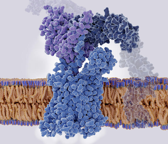
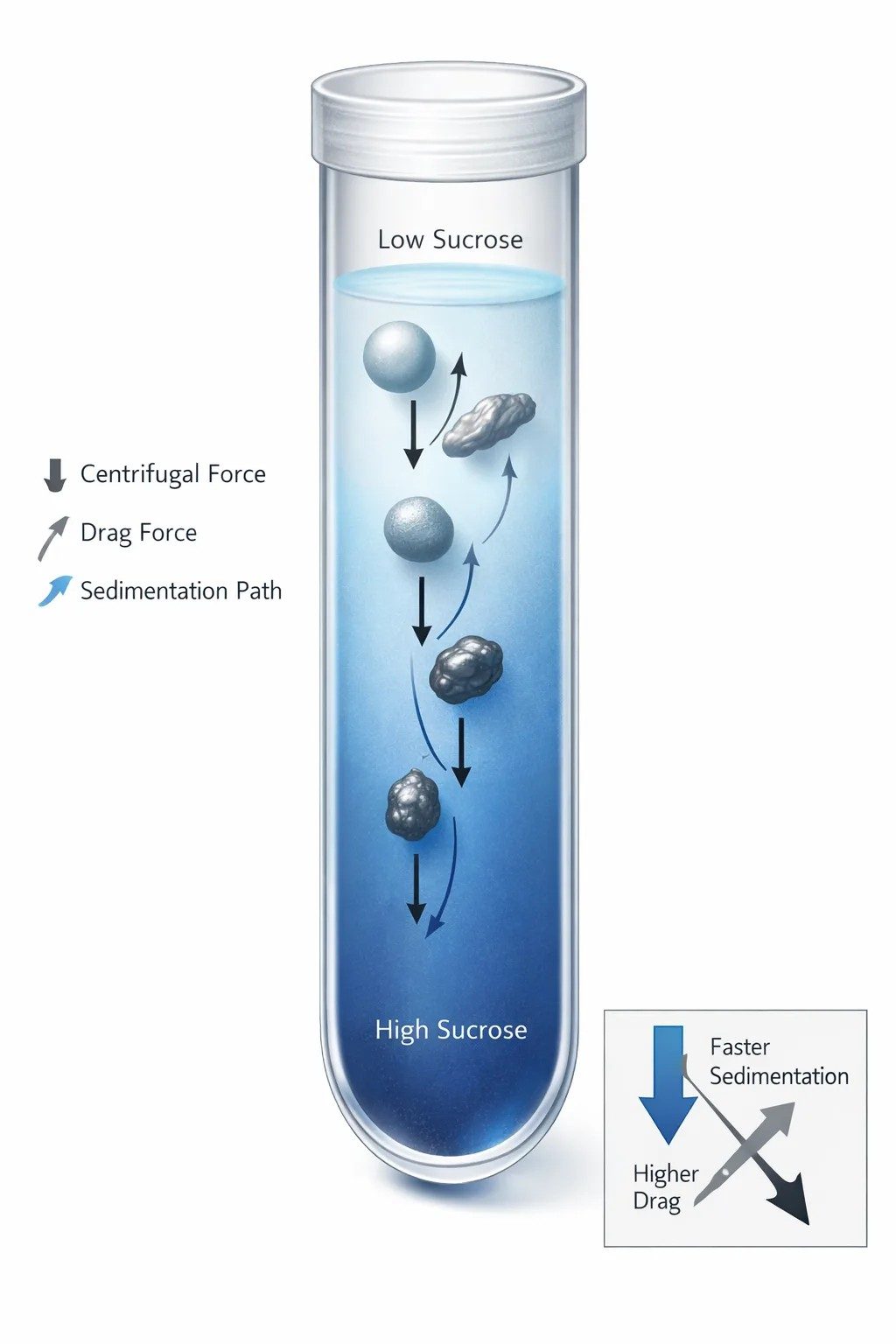 Figure 1: Sedimentation e gradient
Sedimentation in a sucrose gradient is controlled by the balance between driving force, buoyancy, and viscous drag. Nominal size alone is not enough once particle shape and hydration begin to alter friction.
At the simplest level, sedimentation velocity can be described as a balance between three competing effects. The centrifugal field drives the particle outward. Buoyancy offsets part of that force because the surrounding medium has its own density. Viscous drag opposes motion and increases as the medium becomes more resistant. In the familiar Stokes-type picture for a sphere, velocity rises with particle size, rises with the density difference between particle and medium, and falls as viscosity rises.
That framework is still useful. In fact, it remains the cleanest starting point for understanding why gradients work at all. A sucrose gradient does not merely hold the sample in a tube. It changes the local drag and buoyancy terms as the particle moves, which means the medium itself becomes part of the separation mechanism.
The limitation appears as soon as the particle stops being ideal.
A rigid sphere is mathematically convenient because its drag term is well defined. Most research samples are not so cooperative. A ribosomal subunit is asymmetric. An extracellular vesicle may appear round in cartoons but still behave as a hydrated and compositionally variable object. A viral particle may be compact, partially filled, or mechanically perturbed. Protein assemblies can be elongated, flexible, or partially associated. Once the particle departs from ideal geometry, the simple "bigger sinks faster" intuition starts to fail.
This is why the sedimentation coefficient is more informative than diameter alone. The sedimentation coefficient is a transport descriptor. It tells you how the particle actually behaves in the field, not just how large it looks on a schematic. It reflects how strongly the particle is driven and how strongly that motion is resisted by the solvent.
That distinction matters in rate-zonal work because the method separates particles by travel history over time, not by one static property. Two particles can have overlapping nominal sizes and still band apart if one is more compact and the other is more hydrated or more elongated. The root cause is not always a large density difference. Often it is a friction difference.
A short definition helps here. The frictional ratio, written as (f/f_0), compares the effective friction of a real particle with the friction expected for an ideal sphere of the same anhydrous volume. If the ratio is near 1, the particle behaves more like a compact sphere. If it rises above 1, the particle is experiencing extra drag. That extra drag may come from asymmetry, hydration, surface roughness, or conformational looseness. The operational consequence is simple: the particle sediments more slowly than a compact model would predict.
This is one of the main reasons generic protocol language can be misleading. Many pages say that rate-zonal centrifugation separates by size and shape. That is not false. It is just not the level at which a method becomes predictive. The deeper statement is that shape changes hydrodynamic friction, friction changes the sedimentation coefficient, and the sedimentation coefficient controls how far the particle can move before diffusion broadens the band or the particle overruns the gradient.
That logic becomes even more important when the sample contains closely related populations. Consider extracellular vesicle preparations. Small vesicles, membrane fragments, protein-rich particles, lipoprotein-like contaminants, and partially collapsed vesicles can occupy overlapping nominal size ranges. Yet they do not all move the same way. Their frictional behavior differs, and that difference changes how they spread through the gradient. The same is true for ribosomal samples that contain intact particles, subunits, assembly intermediates, or loosely associated factors. In those cases, the gradient is not separating "large from small" in a crude sense. It is resolving a distribution of effective sedimentation coefficients.
There is another layer to this. Even when a particle is close enough to ideal for Stokes-type reasoning to remain useful, its velocity is still not constant during the run. Once it enters a sucrose gradient, it is no longer moving through one medium. It is moving through a sequence of local environments. As depth increases, density rises and viscosity rises with it. The buoyancy term shrinks because the medium becomes denser. The drag term rises because the medium becomes more viscous. So the same particle slows down simply by entering deeper regions of the same gradient.
This is why gradients sharpen banding. They retard motion as the run progresses. A fast particle is allowed to move, but not indefinitely at its starting velocity. The deeper it goes, the more resistance it meets. That retarding behavior helps prevent immediate pelleting and gives neighboring species time to separate spatially.
It also explains why run time is not just an instrument setting copied from another paper. In a good rate-zonal method, time is part of the physical design. If the run is too short, nearby species have not traveled far enough to separate into distinct bands. If the run is too long, the fastest class pushes too close to the bottom while slower bands broaden by diffusion. The best run time is the window in which transport differences have been amplified but not yet erased by overrun or excessive band widening.
A useful rule follows from this. If the target is a real biological assembly rather than an ideal bead, then nominal size should never be the only design variable. The separation should be planned around a practical sedimentation window. That window is shaped by mass, particle density, compactness, hydration, asymmetry, and the local resistance of the medium.
Once that idea is clear, the next step is unavoidable. You cannot optimize the method by asking only which sucrose percentages are popular. You have to ask how the gradient changes velocity with depth.
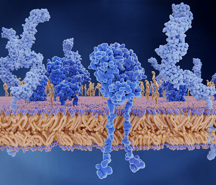
A sucrose gradient is not passive support. It is an active transport field
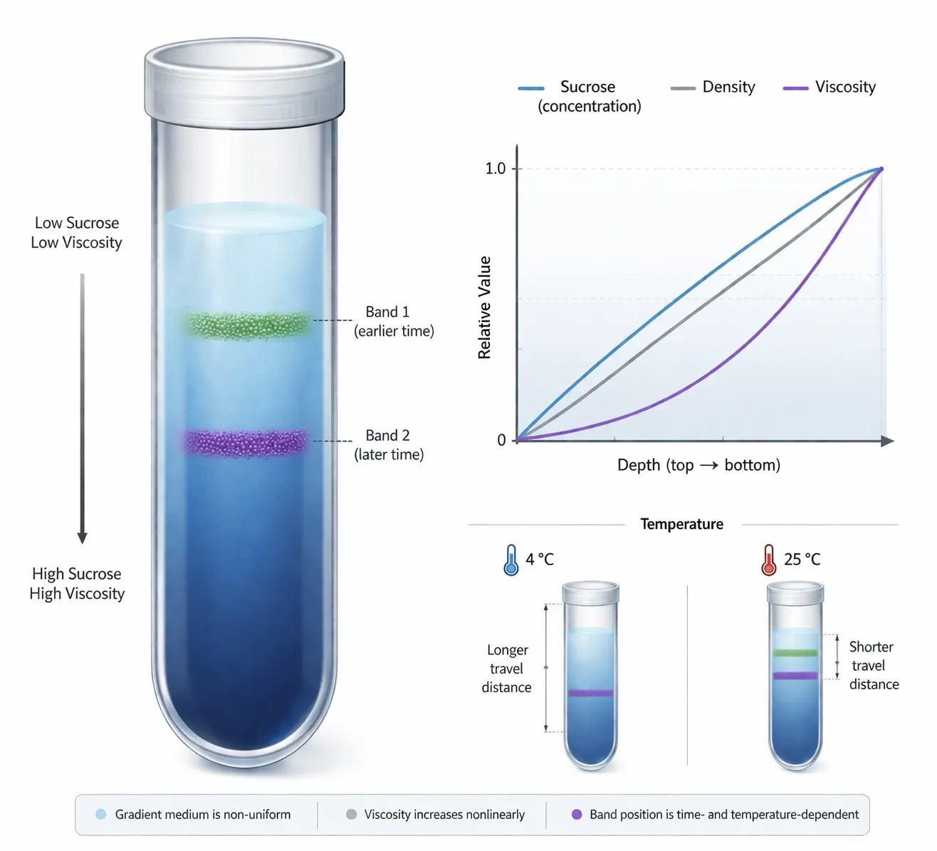 Figure 2: Density–viscosity coupling across a sucrose gradient
In a sucrose gradient, density and viscosity rise with depth and continuously reshape particle transport. Viscosity is not a background property. It becomes an active design variable.
A sucrose gradient does three jobs at once. It establishes a density ramp. It establishes a viscosity ramp. And it damps convective instability. All three functions matter. Yet in routine lab practice, only the density range is usually discussed as if it were the whole design.
That shortcut is one reason many separations remain empirical.
McEwen's classic work on sedimentation through linear sucrose gradients is still important because it forced the problem into the right frame. A particle does not travel through a uniform solvent and then somehow "experience" a gradient at the end. It is retarded continuously by the gradient as it moves through it. That means particle position after a run is the result of integrated transport through a changing medium, not one constant-velocity event with a later correction.
The design consequence is substantial. Density and viscosity are coupled, but they do not influence motion in the same way. As density rises, the density difference between particle and medium becomes smaller, so the net driving force falls. As viscosity rises, drag increases directly. When both increase together, the particle decelerates with depth. Sometimes that deceleration is moderate. Sometimes it is steep enough to decide whether two neighboring bands resolve or collapse.
This is why two gradients with the same nominal top and bottom percentages can still perform differently. A shallower gradient may let fast species enter too easily and separate poorly in the upper half. A steeper gradient may retard them more effectively, but at the cost of slower passage and greater diffusion pressure on slower neighbors. The correct choice therefore depends on the spread of sedimentation behavior in the actual sample, not on habit.
The mistake is to think only in concentration space. The better approach is to think in transport space. Ask what the particle experiences as it descends. How quickly does local viscosity rise? At what depth does the medium density begin to cancel too much of the useful driving force? Does the gradient provide enough retardation to spread neighboring species without trapping the slowest fraction too close to the top?
This is also where temperature stops being a background condition and becomes a method parameter.
Many protocols specify 4°C as if it were just a sample-protection habit. That is too narrow a view. Temperature changes viscosity, and viscosity changes drag. So a temperature change changes the resistance profile of the gradient even when the written recipe is identical. A run that resolves cleanly at one temperature can lose resolution at a warmer condition because the particle sees less drag and penetrates more deeply in the same time window. The reverse can also happen. A colder gradient can hold fast particles higher than expected, leading the operator to extend the run and accidentally broaden slower bands.
That is why "run at 4°C" should be treated as part of the physical identity of the method. Change the temperature and you have changed the gradient in operational terms, even if the sucrose percentages are unchanged on paper.
A useful mental model is this: rotor speed sets the driving field, rotor radius determines how that field is expressed along the path, the gradient sets how drag and buoyancy evolve with depth, and temperature shifts the viscosity landscape beneath the entire run. Only when all four are aligned does a method become transferable.
This helps explain why borrowed protocols often fail across instruments. A lab copies the same sucrose range, the same nominal RCF, and the same time. Yet the bands do not appear in the same places. The immediate assumption is usually that the sample is different. Sometimes that is true. Often the real issue is that the particles are not experiencing the same transport history because the rotor path, thermal behavior, or acceleration and deceleration programs are not equivalent.
A more reliable way to design the gradient is to work backward from band behavior. First, define the target fraction and the nearest neighbor that must be separated from it. Second, define the fastest class that must not pellet during the run. Third, choose a gradient whose upper region allows clean entry, whose middle region spreads the zones, and whose lower region slows the fastest class before bottom overrun. This is not abstract theory. It is the design logic that makes later sample cleanup and preparation workflows and gel-based fraction readouts more interpretable.
A short design workflow makes that logic easier to apply.
A practical design workflow for gradient span, rotor, and run time
Step 1: Define the target and its nearest neighbor.
Do not begin with a stock gradient recipe. Begin with the separation question. Which particle class are you trying to enrich, and which adjacent class is most likely to co-migrate with it? That nearest neighbor determines how much spatial spreading the method must create.
Step 2: Define the must-not-pellet class.
In rate-zonal work, the fastest particles create a hard boundary for run time. If the fastest class reaches the bottom, the system is no longer behaving like a clean zone separation. Before choosing speed or time, decide which species must remain suspended within the gradient at the end of the run.
Step 3: Choose rotor geometry and braking policy before fine-tuning the gradient.
Gradient design is not independent of hardware. A long, orderly sedimentation path supports different band development than a short, wall-biased one. The same is true for stop conditions. If the brake setting is not compatible with narrow zones, fine optimization of gradient percentages will not rescue the method.
Step 4: Match gradient span and run time to the transport window.
Once the target, nearest neighbor, and must-not-pellet class are defined, choose a gradient that provides enough retardation to separate neighbors while keeping the fastest class above the bottom. Then adjust time to maximize spatial spread without pushing the run into overrun or diffusion-dominated broadening.
That sequence looks simple, but it prevents a common mistake: changing everything at once. If the first run is poor, many operators change gradient range, spin time, and rotor speed together. That destroys interpretability. A better approach is to decide whether the failure came from entry, transport, or stopping, then change the variable that governs that stage.
A compact run-time guide also helps.
Run-time interpretation in rate-zonal design
| Run outcome | What the band pattern usually means | First variable to adjust |
|---|---|---|
| Too short | Neighboring species remain compressed near the upper or middle gradient; spacing is limited | Extend run time modestly before changing gradient span |
| Near optimal | Bands are spatially distinct, still suspended within the gradient, and not visibly compressed at the bottom | Preserve time and refine only one secondary variable if needed |
| Too long | Fast species approach the bottom, lower bands compress, slower bands broaden, or recovery becomes ambiguous | Shorten run time or strengthen lower-zone retardation |
This is the point where the method begins to feel less like an inherited protocol and more like a controllable system.
Sample loading still matters, of course. So does sample amount. Overloading is not merely a capacity issue. It changes the hydrodynamic conditions at the top of the gradient and makes early broadening more likely. Underloading creates the opposite problem. It preserves sharpness but may leave too little material for confident fraction detection. The right loading amount is therefore the amount that remains measurable after fractionation without turning the starting zone into a mechanically unstable slab.
That same logic applies to buffer compatibility. Salts, detergents, or residual sample-carrier components can alter local density and viscosity right at the entry layer. The operator may see a neat meniscus and assume the loading step was successful. Meanwhile, the particle enters a local environment that no longer matches the written gradient design.
As shown in Figure 2, viscosity is not a background property that can be ignored until recovery. It changes transport from the moment the particle begins to move. That is why gradient optimization is not solved by percentage tables alone.
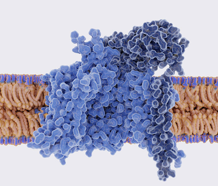
Rotor geometry determines whether the gradient behaves like a clean column or a compromised path
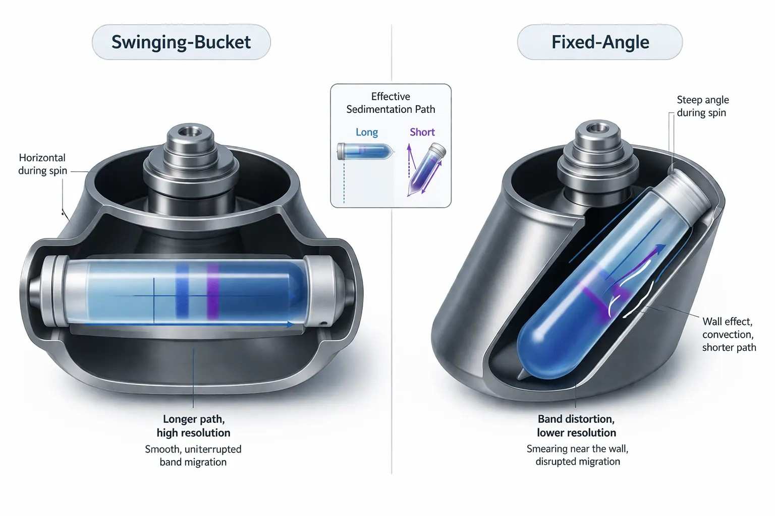 Figure 3: Swinging-bucket versus fixed-angle rotor geometry
Rotor geometry changes effective sedimentation path length and wall interaction. The same nominal RCF does not guarantee the same transport history.
A rate-zonal separation does not occur in an abstract column. It occurs inside a rotor geometry that changes the length, direction, and mechanical quality of the sedimentation path. This is one of the reasons high-resolution work so often favors swinging-bucket rotors over fixed-angle rotors.
The point is not brand preference. It is path geometry.
In a swinging-bucket rotor, the tube swings outward during the run and the gradient aligns into a long working path. The particle moves through that path in a way that is much closer to the column logic assumed in classical gradient design. Bands have room to spread. The route is orderly. Wall-driven interference is reduced.
In a fixed-angle rotor, the situation changes. The path is shorter and oblique. Particles are driven toward the outer wall earlier in the run. That does not make the rotor unusable, but it does make the separation less forgiving when narrow zones matter. The particle is no longer traveling through the most ideal central path for as long. Boundary interaction becomes more important. Band development can become less uniform.
This is where the so-called wall effect becomes useful as a practical term. It does not need to sound mystical. It simply describes the fact that motion near the tube wall is not equivalent to motion in the free central column. Once the sedimentation path is compressed toward the boundary, the band experiences a different local environment. The result can be smearing, altered path length, and lower resolution than the nominal RCF would suggest.
A short explanation helps here too. The rate-zonal regime means a timed separation in which particles are resolved by how far they move before the run stops, not by where they would eventually reach density equilibrium. That regime depends on preserving an orderly path. The more the rotor geometry distorts that path, the harder it becomes to maintain clean rate-zonal behavior.
This is why protocol transfer between rotor types often disappoints. Researchers keep the same written gradient, the same spin time, and the same nominal force. Then they expect the same band map. But the particles are not traveling through the same geometry. Even if the reported RCF matches, the effective transport history can still differ enough to shift spacing, wall interaction, and collection order.
That does not mean fixed-angle rotors have no role. They can be useful for faster, coarser, or more robust separations where the main goal is enrichment rather than narrow discrimination. But when the target is a closely spaced set of macromolecular assemblies, a swinging-bucket rotor usually gives the method more physical room to succeed.
The key point is that rotor choice should be made before troubleshooting begins, not after. If the design goal is high-resolution fractionation, the geometry needs to support that goal from the outset. Trying to rescue a wall-biased path by endlessly adjusting sucrose percentages is rarely the most efficient route.
The remaining resolution losses do not come from sedimentation theory alone. They appear at loading, during deceleration, and again at fraction recovery, where a well-formed gradient can still be degraded by avoidable fluid disturbance.
Sample layering and droplet sedimentation decide whether the run starts narrow or starts broad
The next resolution loss happens before the rotor reaches full speed. It begins at the top of the tube, where the sample first meets the gradient.
In a well-set run, the sample forms a thin starting zone above the least dense part of the gradient. That interface should stay quiet. It should not sink, break, or curl into the upper layer. When the interface remains stable, most particles begin from nearly the same axial position. When it fails, the experiment starts with built-in band broadening.
This is why sample layering is not a cosmetic step. It is the first transport event in the method.
The main variable is the density relationship between the sample carrier and the top gradient layer. If the sample is denser than the top layer, the applied droplet has both downward momentum and a buoyancy advantage. Instead of resting on the interface, it can penetrate it. Once that happens, the sample is no longer a narrow starting band. It becomes a disturbed starting volume.
That distinction matters because every later process acts on the starting width. Sedimentation separates. Diffusion broadens. Convection distorts. If the sample begins as a wide zone, the rest of the method must first overcome loading damage before it can produce useful separation.
A practical loading rule follows from that physics. Keep the sample density close to, or slightly below, the top layer. Apply slowly, with minimal fall distance, and let the liquid spread along the wall rather than inject downward into the column. Multiple protocols for sucrose gradients make the same point operationally by instructing users to place the pipette tip in the meniscus or against the tube wall and layer slowly onto the top of the gradient. Low- or zero-deceleration settings are often paired with that same careful loading logic in swinging-bucket workflows.
Sample volume matters for the same reason. A large load does not just challenge capacity. It creates a thick starting layer. Even if that layer looks visually clean, particles are no longer beginning from one narrow plane. They are beginning from a broader vertical span. That reduces downstream sharpness.
This is one reason upstream handling and downstream readout should be planned together. A gradient prepared for exosome proteomics, exosome lipidomics, or exosome untargeted metabolomics needs a reproducible entry zone, because a noisy load creates ambiguity that later omics data cannot correct.
A second risk sits at the interface chemistry itself. Residual salts, detergents, or carrier components can alter local density and local viscosity right where the sample enters. The meniscus may still look neat. The transport field may already be wrong.
The simplest diagnostic clue is repeatability. If repeated runs under the same spin conditions give similar band depths but inconsistent band widths, the first suspect is often the loading interface, not the rotor.
Deceleration and Coriolis-related remixing can damage a good gradient after the separation looked finished
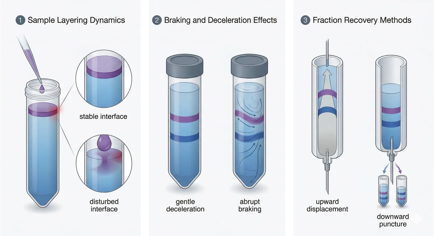 Figure 4 highlights why loading, stopping, and recovery must be treated as part of the separation rather than post-separation handling.
Many users think the separation ends when the band reaches the right depth. It does not. It ends only when the gradient has stopped moving without internal remixing.
During the run, the column exists in a rotating frame. The gradient, suspended bands, and residual fluid structure are all conditioned by that state. If the rotor decelerates too quickly, the liquid does not instantly become motionless. Internal shear and secondary flow can develop while the system relaxes. Narrow zones can tilt, smear, or partially remix before the tube is ever removed from the rotor.
This is the practical meaning of Coriolis-related remixing in rate-zonal work. The term is useful because it captures the fact that fluid parcels in a decelerating rotating system can be deflected into secondary motion. In a gradient tube, that secondary motion is destructive because the method depends on preserving layered order. The exact pattern depends on tube geometry, gradient steepness, and viscosity, but the operational consequence is the same: abrupt braking can broaden bands that were well resolved a minute earlier.
That is why low deceleration or zero deceleration is so common in real sucrose-gradient protocols. It is not folklore. It is a way to let the column relax without forcing internal circulation. Public protocols and technical summaries for polysome and linear sucrose gradients explicitly call for low deceleration or zero deceleration in swinging-bucket rotors, which matches the physical expectation that narrow zones are sensitive during the stop cycle.
A typical failure pattern looks like this. The run time and speed are correct. The gradient appears visually intact. Yet adjacent fractions overlap more than expected, especially in the upper or middle part of the column. That pattern often tempts users to spin longer on the next attempt. But if the real failure happened during braking, a longer run does not solve the problem. It simply pushes the fastest class closer to the bottom and makes the fraction map harder to interpret.
The practical fix is simple. Treat braking as a method variable. Record it. Transfer it with the protocol. Validate it when moving between instruments. A copied RCF is not a copied method if the stop profile changed.
Recovery physics: the fraction collector can preserve the column or stretch it apart
Once the rotor stops cleanly, recovery becomes the next fluid-mechanical event.
The two classical strategies are upward displacement and downward puncture or withdrawal. In upward displacement, a denser solution enters from below and lifts the gradient upward so fractions are collected from the top. In downward withdrawal, the bottom is punctured or sampled so the lowest fractions leave first.
Neither method is universally superior. Each has its own failure mode.
Upward displacement is attractive when preserving band order matters most. If the displacement fluid is introduced smoothly and at the correct density, the column can be translated upward with limited disturbance. The main risk is pulsation from below. A pulsed or overpressurized push can deform closely spaced lower bands.
Downward withdrawal offers direct access to dense lower fractions, but it demands careful flow control. If the withdrawal rate is too high, the column can stretch, entrain neighboring zones, or generate local mixing at the outlet.
The right method depends on where the target band sits and how narrow it is. If the fraction will be used for broad follow-up, moderate widening may be tolerable. If the fraction is intended for fine molecular comparison, collection geometry matters much more. A band heading into protein identification follow-up or label-free quantification may tolerate some overlap. A band intended to distinguish neighboring vesicle or assembly classes usually cannot.
Absorbance profiles should also be interpreted carefully. A smooth A254 or A280 peak does not, by itself, establish compositional or morphological homogeneity of the recovered fraction. It only shows where signal-bearing material is concentrated.
That is why physical recovery should be linked to orthogonal verification. A tracing profile tells you where material is. Composition-focused assays tell you what is enriched. Morphology tells you whether the recovered particles retain the expected structure for the target research fraction. For vesicle-rich or capsid-rich fractions, negative-stain electron microscopy remains a useful confirmatory tool because it directly visualizes morphology after fractionation. Thermo Fisher's technical note on exosome ultrastructural analysis is one example of negative staining being used to examine recovered vesicle structure.
That verification step matters because centrifugation itself can alter particle presentation. High-speed centrifugation has been reported to induce extracellular-vesicle aggregation, which is exactly the kind of artifact that can make a clean-looking fraction harder to interpret if morphology is never checked.
Troubleshooting matrix: convert the physics into first-pass decisions
| Observed issue | Likely physics cause | Change first | Avoid changing first |
|---|---|---|---|
| Broad top fractions | Unstable loading interface or thick starting zone | Improve density match at the top layer and reduce loading disturbance | Max RCF |
| Fast band too close to bottom | Gradient too shallow in the lower half or run time too long | Shorten run time or increase lower-zone retardation | Sample buffer |
| Bands overlap after collection but looked acceptable in the tube | Abrupt braking or aggressive fraction recovery | Lower brake intensity and slow collection flow | Gradient percentages |
| Poor reproducibility across nominally identical runs | Variable loading geometry, sample carrier mismatch, or inconsistent deceleration | Standardize layering technique and stop profile | Rotor replacement |
| Weak signal in all fractions | Underloading or over-fragmented collection scheme | Increase sample concentration or reduce fraction number | Longer spin time |
| Lower bands look compressed | Overrun into the dense end of the gradient | Shorten the run or strengthen early-zone resolution instead of late-zone depth | More sample volume |
The point of this matrix is not to replace judgment. It is to stop the most common troubleshooting mistake, which is changing the gradient, the time, and the speed all at once.
Gradient media comparison: choose the medium for the transport question, not by habit
| Parameter | Sucrose | CsCl | OptiPrep (iodixanol) |
|---|---|---|---|
| Primary logic | Timed transport through a retarding field; widely used for rate-zonal work | Buoyant-density separation; strongly associated with equilibrium banding | Flexible; used in density and velocity-style workflows depending on design |
| Density range | Moderate | High | Moderate to high |
| Viscosity | Relatively high and rises strongly with concentration | Lower than concentrated sucrose in many practical workflows | Generally lower than sucrose at matched useful densities |
| Osmotic behavior | Can become osmotically demanding at higher concentrations | High ionic environment | Often closer to iso-osmotic over useful density ranges |
| Strength | Familiar, robust, and physically good at retarding fast particles | Strong density resolution for equilibrium-style separations | Lower viscosity and gentler osmotic conditions can support morphology retention |
| Main limitation | Less ideal when osmotic load or low-viscosity recovery is the primary concern | Not a drop-in substitute when the real goal is rate-zonal transport control | May not reproduce classical sucrose behavior even when the density range looks similar |
| Best fit | Classical macromolecular fractionation, ribosomes, viral assemblies, vesicle-rich preparations | Density-based discrimination such as full/empty or buoyant-density differences | Fragile assemblies and EV-focused workflows where gentler conditions matter |
Sucrose remains widely used because it is physically forgiving and historically well mapped. Its viscosity profile can help slow particles before pelleting, which is why it remains attractive for classical rate-zonal separations.
CsCl sits in a different category. It is excellent when the question is buoyant density, not simply transport through a gradient. Technical materials describing CsCl workflows for viral preparations emphasize its role in separating particles by density, including full versus empty capsids, which is conceptually different from timed rate-zonal banding.
Iodixanol deserves attention when morphology retention and lower-viscosity handling matter. Multiple sources describe iodixanol as capable of forming iso-osmotic solutions across useful density ranges, and practical comparisons note lower viscosity and osmolality than dense sucrose solutions in many fractionation contexts.
The design rule is simple. Use sucrose when timed transport through a retarding field is the point. Use CsCl when density equilibrium is the point. Consider iodixanol when the target is physically delicate and the osmotic and viscosity burden of sucrose becomes a design problem rather than an advantage.
FAQ
What is the main difference between rate-zonal centrifugation and isopycnic centrifugation?
Rate-zonal centrifugation separates particles by how far they travel in a fixed time window. Isopycnic centrifugation separates particles by buoyant density and continues until each class reaches its equilibrium position.
Why do similarly sized particles sometimes band at different depths?
Because nominal size is only part of the transport problem. Shape, hydration, compactness, and density all change friction and therefore change the sedimentation coefficient.
Why is temperature so important in sucrose gradients?
Because temperature changes viscosity, and viscosity changes drag. A gradient run at a different temperature is not physically the same method, even if the written sucrose range is unchanged.
Why are swinging-bucket rotors usually preferred for high-resolution rate-zonal work?
Because they provide a longer and more orderly sedimentation path with less wall-driven distortion. Beckman's density-gradient rotor guidance explicitly notes that swinging-bucket rotors are especially useful for rate-zonal experiments because the longer pathlength distributes bands better.
What are the first variables to check when bands are broad?
Start with loading density match, starting-zone thickness, and brake profile. Those three variables often explain broad fractions more often than rotor speed does.
Can a longer run rescue poor resolution?
Only if the issue is that neighboring species have not yet spread apart. If the real problem is a disturbed interface or braking-induced remixing, a longer run usually makes the map harder to interpret.
Does a sharp absorbance peak prove that the fraction is clean?
No. It shows where the optical signal is concentrated. It does not prove compositional homogeneity or morphology retention.
When should iodixanol be considered instead of sucrose?
When the target is structurally delicate and lower viscosity or more iso-osmotic conditions are important to the design. That is one reason iodixanol is often discussed in EV-focused workflows.
References
- McEwen CR. Tables for estimating sedimentation through linear concentration gradients of sucrose solution. Analytical Biochemistry. 1967;20(1):114-149. DOI:10.1016/0003-2697(67)90271-0
- Cole JL, Lary JW, Moody TP, Laue TM. Analytical ultracentrifugation: sedimentation velocity and sedimentation equilibrium. Methods in Cell Biology. 2008;84:143-179. DOI:10.1016/S0091-679X(07)84006-4
- Lebowitz J, Lewis MS, Schuck P. Modern analytical ultracentrifugation in protein science: a tutorial review. Protein Science. 2002;11(9):2067-2079. DOI:10.1110/ps.0207702
- Schuck P. Size-distribution analysis of macromolecules by sedimentation velocity ultracentrifugation and Lamm equation modeling. Biophysical Journal. 2000;78(3):1606-1619. DOI:10.1016/S0006-3495(00)76713-0
- Laue TM, Shah BD, Ridgeway TM, Pelletier SL. Computer-aided interpretation of sedimentation data for proteins. In: Harding SE, Rowe AJ, Horton JC, eds. Analytical Ultracentrifugation in Biochemistry and Polymer Science. Cambridge: Royal Society of Chemistry; 1992:90-125.
- Graham JM, Rickwood D. Biological Centrifugation. Oxford: BIOS Scientific Publishers; 2001. ISBN: 978-0387915760.
- Théry C, Amigorena S, Raposo G, Clayton A. Isolation and characterization of exosomes from cell culture supernatants and biological fluids. Current Protocols in Cell Biology. 2006;30:3.22.1-3.22.29. DOI:10.1002/0471143030.cb0322s30
- Linares R, Tan S, Gounou C, Arraud N, Brisson AR. High-speed centrifugation induces aggregation of extracellular vesicles. Journal of Extracellular Vesicles. 2015;4:29509. DOI:10.3402/jev.v4.29509
Research-use note: The discussion below is limited to research-use separation design, fraction characterization, and method optimization for macromolecular particles and related assemblies. For research use only. Not for use in diagnostic procedures.