Is Microflow LC-MS Worth Using for Routine Omics and Bioanalysis?

Meta Intent: A practical decision guide for evaluating whether microflow LC-MS can improve sensitivity, reproducibility, and throughput across routine proteomics, metabolomics, and research bioanalysis workflows.

Microflow liquid chromatography–mass spectrometry (LC-MS) uses lower flow rates and smaller-bore columns than conventional analytical-flow LC while retaining more loading capacity than nano-flow systems. It can improve ion utilization, reduce matrix suppression, and conserve sample. Whether it improves a routine workflow, however, depends on sensitivity, reproducibility, throughput, and method-transfer constraints.

For laboratories deciding whether to adopt or outsource a microflow workflow, the right question is not “Is microflow better than every other LC format?” It is “Will microflow improve the performance metric that currently limits this project?” This article provides a practical framework for answering that question across routine omics and bioanalysis.

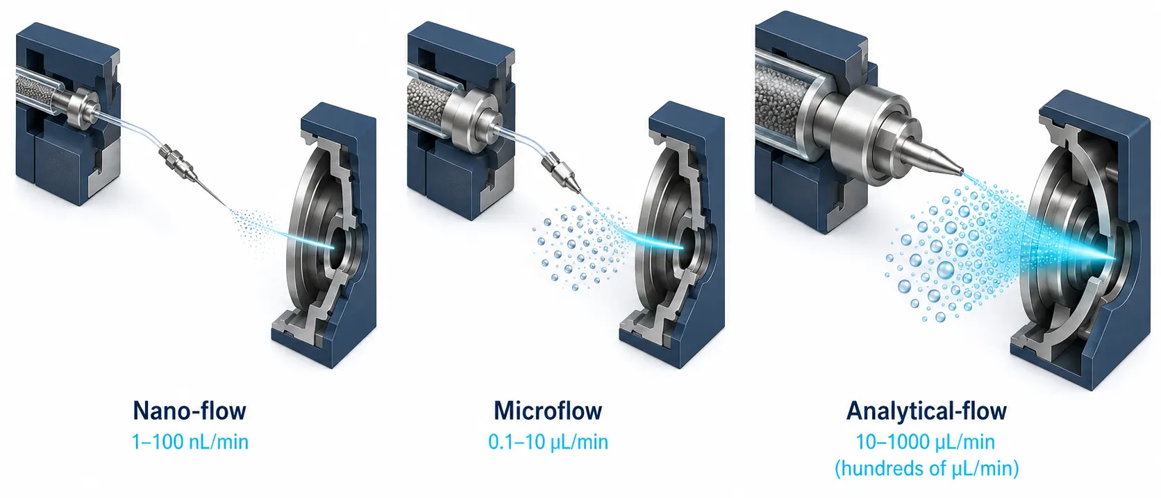
Figure 1: Microflow, nano-flow, and analytical-flow LC-MS interfaces

Caption: Microflow LC-MS is positioned between nano-flow and analytical-flow chromatography. The effective result depends on column internal diameter, flow rate, spray source design, solvent composition, and extra-column volume rather than on flow rate alone.

What Microflow LC-MS Changes at the LC–ESI–MS Interface

Microflow LC-MS uses a smaller-bore column and a lower mobile-phase flow rate than conventional analytical-flow LC. Exact definitions vary by instrument and application, but microflow methods commonly use flow rates in the low microliter-per-minute range and columns with an internal diameter around 1 mm or below. Nano-flow systems operate at substantially lower flow rates, while analytical-flow methods often use 2.1 mm or larger columns and much higher volumetric flow.

The main technical effect of flow reduction occurs at the electrospray interface. A lower liquid flow can generate smaller droplets, which may improve desolvation and increase the fraction of analyte ions transferred into the mass spectrometer. Lower solvent load can also reduce competition among matrix components for charge. In a complex plasma, serum, tissue digest, or metabolomics extract, that change may improve signal-to-noise even when the mass analyzer itself is unchanged.

Microflow can also reduce the amount of sample and solvent required for each injection. This matters when samples are limited, when repeated measurements are needed, or when a study contains many injections. Yet these benefits are coupled to practical constraints. A microflow source needs suitable gas and temperature settings. The column must be loaded within a useful capacity range. Tubing, unions, frits, and the source inlet must be compatible with lower dispersion and lower flow.

For laboratories comparing platforms, a useful starting point is to review the broader Liquid Chromatography (LC) Based Analysis Services landscape and then define the exact analytical bottleneck. Microflow is not a universal replacement for every LC-MS configuration.

The Real Decision: Which Bottleneck Are You Solving?

Adoption decisions become clearer when the workflow is described in terms of constraints rather than instrument categories. Four questions should be answered before changing the flow regime.

First, is sensitivity limiting the study? If the target signal is already well above the required quantitative floor, more ion current may not improve the biological conclusion. If low-abundance species are being lost in matrix background, microflow may be more valuable.

Second, is sample availability limiting the design? Microflow can reduce the amount consumed per injection, but the usable sample load still depends on column capacity, analyte concentration, and the need for replicate or confirmatory injections. A smaller injection volume is not automatically a better experiment if it increases sampling error.

Third, is the project limited by batch size? A system that provides excellent single-injection sensitivity but requires frequent troubleshooting may be less useful for a large cohort than a slightly less sensitive system that maintains stable retention time, peak area, and carryover performance.

Fourth, how much method-transfer risk is acceptable? Changing from analytical flow to microflow can require new source conditions, gradient timing, column dimensions, injection settings, and system-suitability criteria. A laboratory that needs to preserve a validated routine workflow may value transfer simplicity more than peak signal.

This is why the Ultra Performance Liquid Chromatography (UPLC) Based Analysis Service should be treated as a related analytical option rather than an automatic competitor. The relevant comparison is between complete workflows, not isolated flow-rate values.

Sensitivity: When Microflow Can Improve the Quantitative Floor

The clearest case for microflow occurs when ionization efficiency or matrix suppression is the limiting step. Smaller electrospray droplets can improve desolvation and ion formation, while lower solvent flow can reduce the number of co-eluting matrix molecules entering the source at the same time. The result may be a higher signal-to-noise ratio, better peak detectability, or an improved lower limit of quantification.

The size of the benefit depends strongly on the analyte and matrix. A clean standard solution may show only a modest difference, while a plasma extract, tissue digest, or highly concentrated metabolomics matrix may show a more meaningful change. Analyte polarity, charge state, surface activity, adsorption tendency, and source temperature can all influence the result.

Sensitivity should therefore be evaluated with more than peak height. A paired comparison should record signal-to-noise ratio, peak area, matrix factor, recovery, calibration linearity, precision, accuracy, and the lower limit of quantification. If a microflow method increases peak intensity but also increases variability or causes source saturation at the upper end of the calibration range, its practical value may be smaller than expected.

The Mass Spectrometry Platform must also be considered. The same LC flow regime can behave differently with different source geometries, gas controls, inlet designs, and mass analyzers. A valid comparison should keep the MS platform and data-processing logic as constant as possible while optimizing only the parameters that must change for microflow.

Figure 2: Sensitivity and matrix-effect evaluation

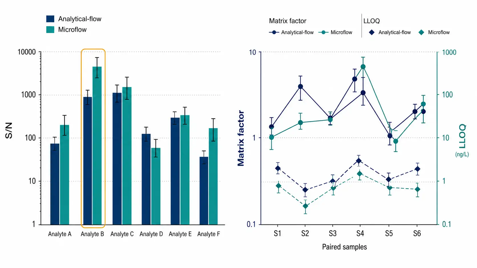
Caption: A decision-oriented sensitivity plot should compare signal-to-noise, matrix factor, calibration range, and lower-limit performance rather than showing signal intensity alone.

For protein workflows with very limited material, the sample strategy is equally important. A resource such as Micro-Sample Protein Quantification Techniques can help frame the relationship between available material, sample preparation losses, and the amount ultimately loaded onto the LC column. Microflow may preserve more signal, but it cannot recover analyte that was lost during extraction, digestion, cleanup, or transfer.

Reproducibility: Evaluate More Than a Single Good Injection

Routine analysis is defined by repeated performance. A microflow system should therefore be assessed with batch-level metrics rather than one representative chromatogram.

Retention-time reproducibility is important for targeted assays, alignment, and scheduled acquisition. Peak-area reproducibility determines whether quantitative differences are biological or technical. In discovery proteomics, identification consistency and missing-value rates are also relevant. For complex matrices, carryover, blank response, source contamination, and QC drift can become more important than the signal gain observed in the first few injections.

A useful qualification set includes system-suitability injections, blanks, pooled QC samples, matrix-matched standards, and representative study samples. The same samples should be distributed across the beginning, middle, and end of a batch. This design can reveal gradual pressure increase, source fouling, retention-time drift, or changes in peak shape that are invisible in a short test.

Microflow may improve reproducibility because a wider column is less vulnerable to overloading than a narrow nano-flow column. It can also lower carryover in some high-complexity proteomics workflows because the column capacity and solvent volume are better matched to the injected material. These are method-dependent advantages, not guarantees.

In one large-scale microflow proteomics study, chromatographic retention-time CV remained below 0.3% and protein quantification CV remained below 7.5% across more than 2,000 samples. These values should be treated as study-specific benchmarks rather than universal acceptance criteria.

Figure 3: Batch-level reproducibility dashboard

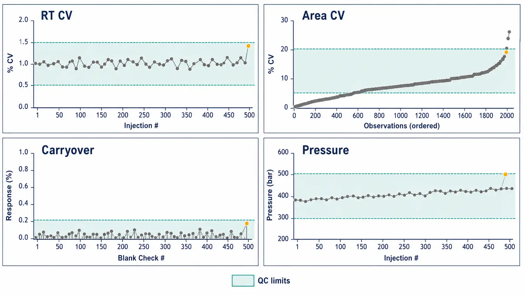
Caption: A modern QC dashboard should track retention-time CV, peak-area CV, carryover, pressure, blank response, and identification consistency across the full injection sequence.

The practical question is whether the workflow remains within predefined QC limits over the batch size that matters. A method that is excellent for 20 samples but unstable after 200 injections has not solved a routine-analysis problem.

Throughput: Why Flow Rate Alone Does Not Determine Sample Capacity

Throughput is often described as the number of samples analyzed per hour, but the correct unit is the complete sample cycle. The cycle includes injection, gradient, re-equilibration, wash, blank monitoring, column conditioning, and any time needed for system-suitability checks.

A shorter gradient can increase nominal throughput, but it may also reduce chromatographic separation, increase co-elution, or make the method more sensitive to small changes in flow and temperature. In discovery proteomics, a short method may reduce proteome depth. In targeted bioanalysis, a short method may be acceptable if selectivity and quantitative performance remain within the project criteria.

Sample preparation can dominate the schedule. If extraction, digestion, enrichment, evaporation, or plate handling takes longer than LC-MS acquisition, changing from analytical flow to microflow may have little effect on total project throughput. Conversely, when the instrument is the bottleneck, reduced equilibration time and stable short gradients can make microflow more valuable.

LC-MS workflow capacity should therefore be evaluated by total workflow capacity, not by the LC flow rate printed in an instrument specification. The relevant question is how many samples can pass the full workflow while retaining acceptable QC performance.

Figure 4: Real sample-cycle timeline

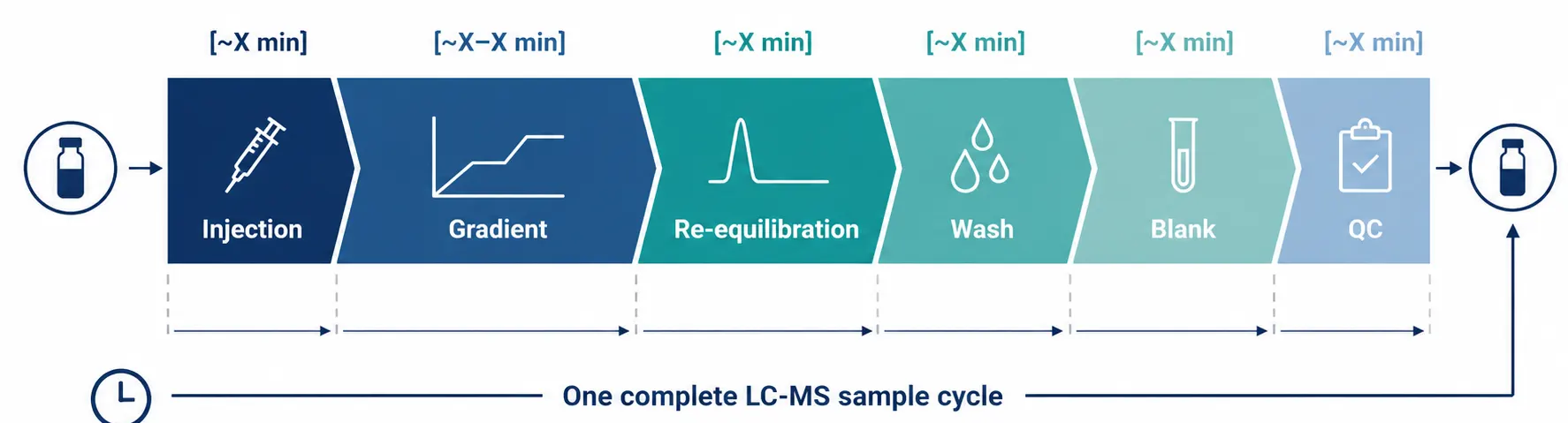
Caption: Effective throughput is determined by the combined duration of gradient, re-equilibration, injection, wash, blank, and QC steps.

Where Microflow Fits in Routine Proteomics and Metabolomics

Microflow is particularly attractive when a project needs more than one of the following: limited sample consumption, stable large-batch measurement, moderate-to-high sensitivity, and compatibility with conventional LC-MS infrastructure.

In bottom-up proteomics, microflow can support label-free quantification, DIA, short-gradient profiling, plasma or serum analysis, and selected phosphoproteomics workflows. The optimum configuration still depends on sample complexity and required depth. A deep discovery experiment with very low input may favor nano-flow, while a large cohort with sufficient digest material may benefit from a more robust microflow format.

For quantitative proteomics, Label-Free Quantification Services for Deep Proteome Profiling and DIA Quantitative Proteomics Service represent different data-acquisition contexts in which LC stability and missing-value control can matter as much as absolute signal.

Label-based workflows introduce another consideration. In TMT Based Proteomics Service, multiplexing can improve the number of biological conditions represented in a run, but the LC-MS method still has to manage co-elution, ratio compression, sample complexity, and batch consistency. Microflow may support throughput, but it does not remove the need for appropriate fractionation, loading, and acquisition design.

In metabolomics, microflow can be considered for untargeted profiling, targeted panels, lipidomics, and complex biological matrices. The decision depends on whether the study prioritizes broad feature coverage, quantitative precision, low sample use, or rapid analysis. A microflow method should not be judged only by the number of detected features. Feature reproducibility, annotation confidence, blank subtraction, pooled-QC stability, and batch correction requirements are equally important.

Figure 5: Application-fit map for LC flow regimes

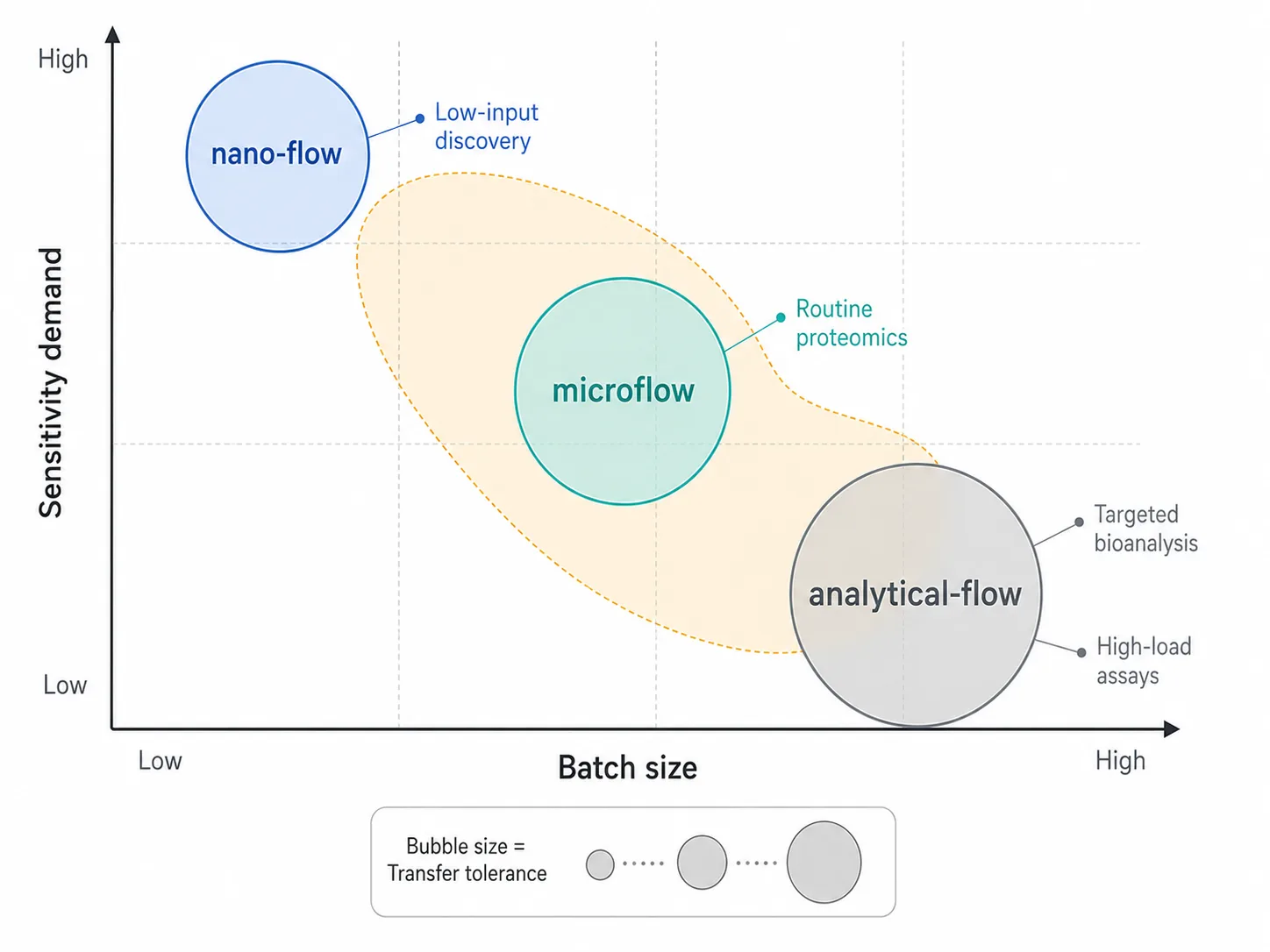
Caption: The application-fit map positions nano-flow, microflow, and analytical-flow LC-MS according to sensitivity demand, sample complexity, batch size, and acceptable transfer risk.

Where Microflow Fits in Targeted Bioanalysis

Targeted bioanalysis often has a different success criterion from discovery omics. The objective is usually reliable quantification across a defined calibration range, not the maximum number of detected features or proteins.

Microflow may be useful for small molecules, peptides, metabolites, and other analytes when matrix suppression limits the lower end of the assay. Lower flow can also reduce solvent and sample consumption. However, the method still needs selectivity, accuracy, precision, stability, dilution integrity, carryover control, and a defensible calibration model.

The source must be optimized for the low-flow regime. Spray voltage, gas flow, source temperature, desolvation conditions, and post-column tubing can influence both sensitivity and peak shape. A source that performs well at analytical flow may not be optimal at microflow without adjustment.

For broader profiling, Targeted Metabolomics Service and LC-MS/MS Untargeted Metabolomics represent different analytical goals. Targeted assays usually emphasize calibration, precision, and quantitative range. Untargeted workflows place greater emphasis on feature coverage, alignment, annotation, and pooled-QC behavior. The same microflow setting should not be assumed to be optimal for both.

In research bioanalysis, microflow is most defensible when the improvement can be demonstrated in a paired design. Compare the existing method and the microflow method using the same sample preparation, analyte set, mass spectrometer, and data-processing rules wherever possible. Then assess whether the gain in the lower concentration range is accompanied by acceptable precision and batch stability.

Method-Development Variables That Decide Whether the Benefit Survives Transfer

Microflow performance is controlled by a network of variables rather than one setting. The most important variables are:

• Column internal diameter, length, particle size, stationary phase, and loading capacity.
• Flow rate, gradient slope, re-equilibration time, and column temperature.
• Injection volume, sample concentration, solvent mismatch, and total sample load.
• Mobile-phase additives, pH, organic solvent composition, and buffer volatility.
• Spray voltage, source temperature, nebulizing gas, drying gas, and inlet position.
• Tubing length, internal diameter, unions, frits, and post-column dead volume.
• Wash solvent strength, blank frequency, carryover criteria, and cleaning strategy.
• MS acquisition mode, cycle time, ion accumulation, scheduled windows, and dynamic range.

The best development strategy is to define acceptable ranges rather than search for one perfect set point. For example, a flow rate that produces the highest signal in a standard may not provide the most stable performance in a plasma matrix. A very steep gradient may increase sample turnover but reduce peak separation. A larger injection may improve detectability until column loading or peak distortion becomes limiting.

Method transfer should also be judged by data equivalence. If the biological interpretation changes because microflow alters missingness, co-elution, ion ratios, or peptide identification consistency, a simple signal comparison is insufficient. The transferred method must be evaluated at the level of the final decision the study will make.

How to Compare Microflow with an Existing LC-MS Method Fairly

An efficient comparison begins with a matched sample set. Use the same biological matrix, the same analyte preparation, and the same internal standards whenever possible. If the comparison changes sample cleanup, digestion, enrichment, or injection volume at the same time as the LC flow regime, the source of the observed improvement becomes difficult to identify.

The mass spectrometer should also remain constant during the first comparison. The purpose of a paired pilot is to isolate the contribution of chromatographic scale and ionization conditions. After that baseline comparison, the microflow method can be optimized for its own source, column, and acquisition settings. This two-stage design separates a fair technology comparison from normal method development.

The data review should be structured around decision thresholds. For a targeted assay, ask whether the microflow method reaches the required lower concentration range with acceptable precision and carryover. For discovery proteomics, ask whether the method improves usable identifications, missing-value behavior, and batch consistency rather than only raw identification count. For metabolomics, ask whether pooled-QC feature stability and annotation confidence improve across the batch.

It is also important to record what does not improve. A microflow method may increase signal but leave the quantitative range unchanged because the assay is limited by recovery or calibration design. It may reduce solvent consumption but add more stringent source cleaning. These tradeoffs should be documented explicitly so that adoption is based on total workflow value rather than a single favorable metric.

Failure Modes: When Analytical Flow or Nano-flow May Still Be Better

Microflow should not be adopted simply because it is newer or because a published study reported a large sensitivity gain. Analytical flow can remain the better choice when the assay already has sufficient sensitivity, when high sample loading is required, or when a validated routine method must be preserved with minimal changes.

Nano-flow can remain preferable when the primary goal is maximum sensitivity from extremely limited input and the laboratory accepts the additional operational demands. It may also be appropriate for deep discovery workflows where proteome depth is more important than large-batch robustness.

Microflow can be a poor fit when the true bottleneck is sample preparation, analyte recovery, chromatographic selectivity, or data interpretation. It can also introduce new risks if the system is not configured for low dispersion and stable low-flow delivery. Increasing sensitivity does not compensate for poor recovery, high carryover, unstable calibration, or inadequate QC.

The most common decision error is to compare a high-performing microflow method with a poorly optimized analytical-flow method. A fair comparison should use matched samples, comparable column chemistry, the same mass spectrometer where possible, and predefined acceptance criteria.

A Practical Go/No-Go Qualification Plan

A small qualification study can establish whether microflow is worth scaling. The design should include the following sequence.

1. Record the current method baseline, including sensitivity, precision, retention-time stability, cycle time, carryover, and sample consumption.
2. Select representative standards, pooled QC material, blanks, and real study matrices.
3. Build a microflow method using the same analyte preparation and MS platform where possible.
4. Optimize only the conditions that must change, such as source settings, flow rate, gradient, and injection volume.
5. Compare signal-to-noise, matrix factor, calibration behavior, precision, accuracy, peak shape, and carryover.
6. Run the methods across the beginning, middle, and end of a representative batch.
7. Calculate total cycle time, including wash and re-equilibration rather than gradient time alone.
8. Set a Go/No-Go decision based on the project’s real priorities.

The outcome may be full adoption, adoption for selected workflows, retention of the existing flow regime, or additional optimization. A mixed strategy is often reasonable: microflow for large-batch or matrix-limited work, nano-flow for ultra-low-input discovery, and analytical flow for established targeted assays.

Figure 6: Microflow LC-MS qualification workflow

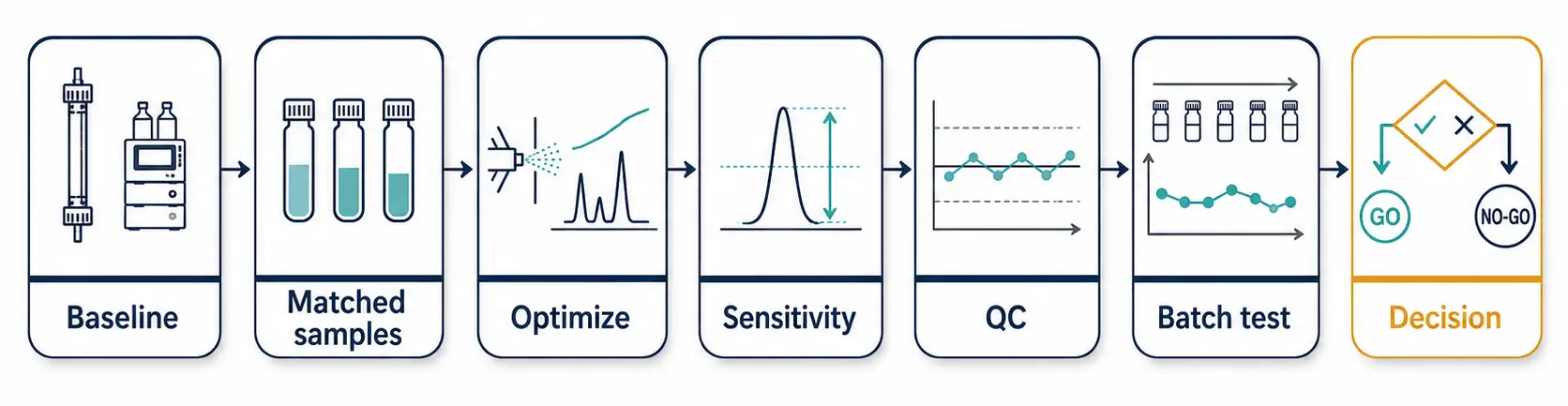
Caption: The qualification workflow compares matched methods using sensitivity, reproducibility, carryover, batch stability, sample use, and full cycle time before adoption.

Final Decision: Is Microflow LC-MS Worth It?

Microflow LC-MS is worth serious consideration when a laboratory needs a better balance between sensitivity and operational stability. It is especially attractive when sample is limited, matrix suppression is important, or a large batch must be analyzed with consistent retention time and quantitative behavior.

It is less compelling when the current assay already meets its sensitivity requirement, when sample preparation dominates the workflow, or when method-transfer risk is greater than the expected analytical benefit. In those cases, optimizing the existing analytical-flow or nano-flow method may be the more efficient scientific decision.

The most defensible adoption strategy is evidence-based. Use a paired pilot, evaluate batch-level QC, and define success using the metrics that matter to the project. Microflow LC-MS is not a universal replacement for other LC formats. It is a practical workflow option whose value appears when its sensitivity, reproducibility, and throughput advantages match the actual problem being solved.

FAQ

How is microflow LC-MS different from nanoLC?

Microflow LC-MS uses higher flow rates and wider columns than nanoLC, while still operating below conventional analytical-flow conditions. It generally aims to balance improved ionization with better loading capacity and operational robustness.

Is microflow LC-MS suitable for routine quantitative bioanalysis?

It can be suitable when matrix effects, sample availability, or sensitivity are limiting factors. Suitability must be demonstrated through selectivity, accuracy, precision, carryover, stability, and batch-level QC testing.

Does microflow LC-MS always improve sensitivity?

No. The benefit depends on the analyte, matrix, column, source, solvent composition, and operating conditions. A paired comparison is required to determine whether the gain is meaningful for a specific assay.

What should be compared in a microflow LC-MS pilot study?

Compare signal-to-noise, matrix factor, calibration range, precision, accuracy, retention-time stability, carryover, sample consumption, and complete cycle time. Do not compare peak intensity alone.

When is microflow LC-MS not worth adopting?

It may not be necessary when sensitivity is already sufficient, sample preparation is the main bottleneck, or an established analytical-flow method already meets its QC requirements.

How can a laboratory qualify microflow LC-MS before full adoption?

Use matched samples and compare sensitivity, precision, carryover, retention-time stability, sample consumption, and complete cycle time across a representative batch.

References:

1. Bian, Y., et al. “Robust, reproducible and quantitative analysis of thousands of proteomes by micro-flow LC–MS/MS.” Nature Communications. Open access under CC BY 4.0. DOI: 10.1038/s41467-019-13973-x.
2. Fitz, V., et al. “Systematic Investigation of LC Miniaturization to Increase Sensitivity in Wide-Target LC-MS-Based Trace Bioanalysis of Small Molecules.” Open access under CC BY. DOI: 10.3389/fmolb.2022.857505.
3. Seo, Y., et al. “Simple and robust high-throughput serum proteomics workflow with low-microflow LC–MS/MS.” Analytical and Bioanalytical Chemistry. Open access under CC BY 4.0. DOI: 10.1007/s00216-024-05603-3.
4. “Microflow LC-MS Bottom-Up Proteomics Using 1.5 mm Internal Diameter Columns.” ACS Omega. Open access under CC BY 4.0. DOI: 10.1021/acsomega.4c10591.
5. Girel, S., et al. “Hyphenation of microflow chromatography with electrospray ionization mass spectrometry for bioanalytical applications focusing on low molecular weight compounds: a tutorial review.” Open access under CC BY 4.0. DOI: 10.1002/mas.21898.
6. Abele, M., et al. “Unified Workflow for the Rapid and In-Depth Characterization of Bacterial Proteomes.” Open access under CC BY. DOI: 10.1016/j.mcpro.2023.100612.