Far-UV CD Secondary Structure: How Accurate Is It, and How to Avoid Deconvolution Pitfalls

Far-UV CD secondary structure analysis is one of the fastest ways to see whether a protein's fold is intact, shifting, or destabilized. Used well, it's great for trend detection and screening. Used casually, it can mislead. If you're judging Far-UV CD accuracy or reviewing a circular dichroism deconvolution report, this guide gives you practical decision boundaries—so you can decide when a % helix/sheet number is trustworthy and when you should require orthogonal methods.

Key phrases up front: Far-UV CD secondary structure, circular dichroism deconvolution, and Far-UV CD accuracy.

Key takeaways

• Far-UV CD delivers reliable trend detection; absolute percentages depend on wavelength coverage, data quality, and model fit.
• Use a confidence-tier approach (High/Moderate/Limited) combining coverage (190–250 vs 200–250 vs >205–250 nm), QC gates (HT/OD/replicates), and fit diagnostics (NRMSD/residuals).
• Require orthogonal confirmation (FTIR/DSC/DLS/SEC) when coverage is limited, β-rich content is decision-critical, or QC/red flags appear.
• Insist on an auditable package: raw + baseline-subtracted spectra, HT/absorbance indicators, algorithm/reference set disclosure, fit residuals, and a QC summary.

What Far-UV CD can—and can't—tell you about secondary structure

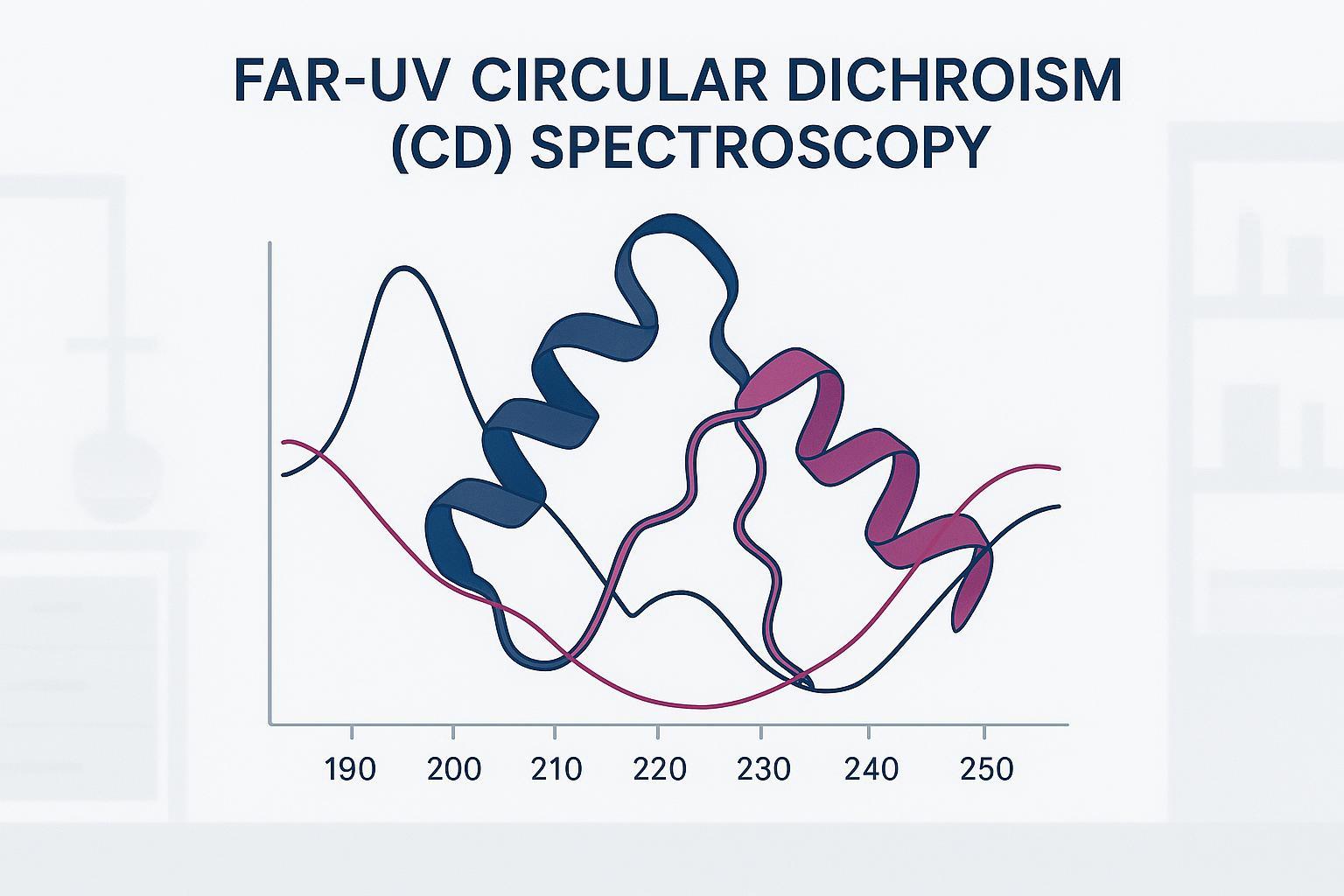
Far-UV CD (roughly 190–250 nm) probes peptide-bond transitions that encode secondary-structure signatures—classic α-helix valleys near 208/222 nm, β-sheet features around 195–218 nm, and "other" elements. It can estimate relative proportions and detect folding changes, but it won't give atomic detail or unambiguously resolve mixed conformations without caveats. Synchrotron radiation CD (SRCD) improves low-wavelength access; most benchtop instruments are buffer- and HT-limited below ~190–200 nm.

For decision-making, treat "accuracy" as conditional: better wavelength coverage improves information content and deconvolution stability; clean baselines and matched blanks prevent artifacts; the chosen algorithm/reference set shapes estimates. At minimum, request a deconvolution report plus a QC summary so you can audit assumptions and data quality.

Decision boundaries, in practice:

• High confidence: 190–250 nm coverage with good QC → accept trend conclusions; report model-based % with uncertainty.
• Moderate confidence: 200–250 nm → accept trends; avoid strong absolute % claims for β-rich/multi-domain proteins; consider FTIR corroboration.
• Limited confidence: >205–250 nm or QC fails → use for screening only; require orthogonals for decision-critical conclusions.

According to a tutorial by Miles and colleagues, careful data collection and transparent analysis significantly improve reliability, and deconvolution must be paired with fit diagnostics and reporting of assumptions. See the peer-reviewed overview in the Chem. Soc. Rev. 2021 tutorial by Miles et al. in the "Tools and methods for circular dichroism spectroscopy".

The Trust Framework: three checks before you believe any % helix/sheet number

Before acting on any CD-derived percentage, run this triage:

1. Spectral quality and wavelength coverage. Confirm usable coverage down to at least 200 nm (190–200 adds valuable information for β-structures), smooth curves, and replicate agreement. JASCO's learning center explains why photons drop at low wavelengths and the detector's high-tension (HT) rises, increasing noise; see JASCO's CD theory overview.
2. Baseline/blank hygiene. Acquire buffer-only spectra under identical conditions and subtract from the sample. Verify a flat overlay above ~250–260 nm and watch for curvature that signals absorbance or scattering. The Miles tutorial emphasizes proper blank matching and baseline subtraction; see the CD best-practice tutorial (2021).
3. Reference set and model fitness. Use established algorithms (SELCON3, CONTINLL, CDSSTR) and suitable reference sets (SP175/SMP180; truncated sets if coverage begins at 190 nm). Report algorithm, reference set name, and fit diagnostics such as NRMSD/RMSD with residual plots. DichroWeb's overview explains these models and datasets; see the DichroWeb documentation and PCDDB overview.

Wavelength range requirements for Far-UV CD secondary structure deconvolution

Lower wavelengths carry more secondary-structure information, but access is limited by buffer absorbance and HT behavior. As photons diminish below ~200 nm, HT rises; once HT approaches ~600–650 V, noise and instability spike, and points shouldn't be trusted. Buffers with poor far-UV transparency (e.g., Tris, imidazole, DTT, high salts, sugars) and long pathlengths can create absorbance walls.

Practically, think in tiers:

• High confidence: 190–250 nm — better β-sheet discrimination and more stable deconvolution.
• Moderate confidence: 200–250 nm — reliable trends; cautious on absolute %.
• Limited confidence: >205–250 nm — use for screening only.

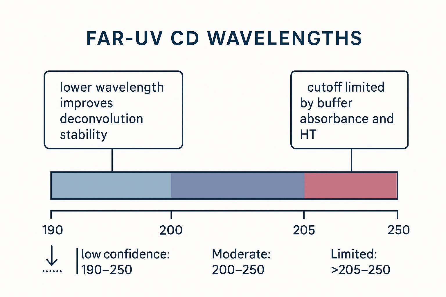
How Far-UV CD wavelength coverage affects secondary structure deconvolution confidence.

For practical sample/buffer planning (UV cutoffs, pathlength choices), see the brand's support page on sample concentration and pathlength planning.

Study design that improves accuracy: pathlength, concentration, replicates, and temperature control

Here's the plan that ties each choice to a failure mode it prevents:

• Pathlength and concentration: Target an optical density (OD) near ~0.9 AU at your shortest wavelength (acceptable ~0.4–1.2 AU; avoid >1.5–2.0 AU) to keep HT comfortably below ~600–650 V. Short-path cells (0.1–1 mm) enable higher concentrations without hitting absorbance walls.
• Replicates and averaging: Acquire 3–10 accumulations per spectrum and average them; increase integration time and adjust bandwidth judiciously to boost SNR without clipping features.
• Temperature control: Use a thermostatted holder to avoid drift across scans; temperature changes shift spectra and can mimic instability.
• Matched blanks: Prepare buffer-only spectra matched to the final sample dilution for accurate baseline subtraction.

For buffer compatibility and UV cutoff guidance, see buffer UV cutoff limits.

Deconvolution workflow explained (without math overload)

Most data paths follow this sequence:

• Preprocess: subtract matched buffer baseline; consider minimal smoothing only with justification.
• Normalize: convert to mean residue ellipticity (MRE) or Δε using accurate pathlength and concentration.
• Choose algorithms: run SELCON3, CONTINLL, and CDSSTR; compare outputs rather than trusting a single model.
• Select reference sets: pick SP175/SMP180 (or truncated versions if starting at 190 nm) that match the protein class; for β-rich proteins, consider BeStSel as a check.
• Fit diagnostics: report NRMSD/RMSD, overlay experimental vs back-calculated spectra, and show residual plots.
• Uncertainty: present ranges or qualitative confidence tiers; state model dependence and data-condition limits.

DichroWeb provides accessible documentation of algorithms and datasets; see the DichroWeb/PCDDB overview and key best practices in Miles et al., 2021.

Choosing algorithms and reference sets: why one protein can give different answers

SELCON3, CONTINLL, and CDSSTR embody different assumptions. SELCON3's self-consistent SVD approach can be robust to moderate noise; CONTINLL uses regularization that can be parameter-sensitive; CDSSTR often performs well for well-folded proteins. Reference sets matter just as much: SP175 (soluble globular proteins) and SMP180 (including membrane proteins) are common choices; truncated sets are used when spectral starts at ~190 nm. For antibodies, recent benchmarking suggests SP175/SMP180 are reasonable starting points, but β-sheet-rich scaffolds and multi-domain architectures magnify model dependence. See a cohort analysis in 2024: Bruque et al. reported mAb deconvolution variability and method comparisons in "Analysis of the Structure of 14 Therapeutic Antibodies".

What to ask your provider:

• Which algorithms and reference sets were used, and why are they appropriate for your protein class?
• Are fit diagnostics (NRMSD/RMSD) reported with overlay/residual plots?
• How do results change across algorithms/reference sets, and what uncertainty language accompanies the outputs?

Quality gates: SNR, HT voltage, absorbance, and red flags in raw spectra

Before deconvolution even starts, apply QC gates and look for "red flags" that reduce Far-UV CD accuracy:

• HT behavior: If HT rises toward ~600–650 V at low wavelengths, photon scarcity increases noise; do not trust points beyond stability. JASCO notes HT-linked noise growth in the far-UV; see JASCO's CD ebook (2020).
• Absorbance limits: Aim for OD ~0.9 AU at the shortest wavelength; accept ~0.4–1.2 AU; avoid >1.5–2.0 AU to prevent HT stress and saturation. Facility guidance from OSTR summarizes practical targets; see Applied Photophysics OSTR guidance.
• Replicates/SNR: Collect 3–10 scans and average; adjust D.I.T./bandwidth as needed to stabilize SNR without distorting features. The Harvard CMI J-815 getting-started guide outlines replication and acquisition practices; see CMI's J-815 guide.
• Baseline mismatch: Non-flat high-wavelength baselines or poor overlay above ~250–260 nm usually signal buffer differences or contamination.

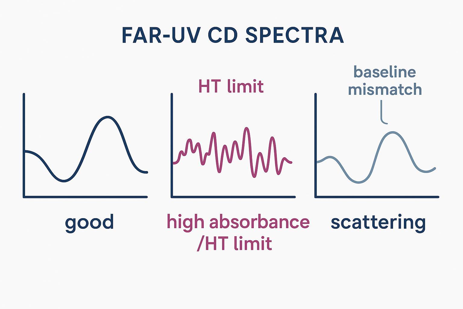
Common Far-UV CD spectral red flags that reduce secondary structure deconvolution accuracy.

For comparison guidance on when to add FTIR or DSC, see our resource on when to add FTIR or DSC.

Scattering, absorbance, and baseline errors: the three pitfalls that mislead deconvolution

• Scattering (aggregates/particles; excipients/high salt): Detect via noisy low-wavelength regions and distorted baselines; fix by centrifugation/filtration (e.g., 10–14k × g, 10–15 min; 0.22 µm filters), optimizing buffer, and checking DLS/SEC for particles. A beginner's guide and reviews note these signatures; see Rodger's beginner's guide to CD (2021).
• Absorbance walls (buffer UV cutoff; too long pathlength): Detect by high OD and rising HT at low λ; fix by shortening pathlength, diluting, and swapping to low-absorbance buffers (e.g., low-concentration phosphate). Best-practice tutorials emphasize buffer transparency; see Miles et al., 2021.
• Baseline mismatch (blank not identical): Detect via non-flat overlay above ~250–260 nm; fix by matching the blank exactly (same buffer, same dilution, same cuvette), re-running scans, and confirming cleanliness. SOP-style guidance appears in facility notes; see CMI's J-815 guide.

Special cases: antibodies, multi-domain proteins, IDPs, and glycoproteins

Some proteins produce reasonable-looking outputs that are still wrong if over-interpreted:

• Antibodies (β-sheet-rich immunoglobulins): Expect model dependence and variability across algorithms/reference sets. Treat absolute % cautiously unless coverage/QC is high; rely on trends and require FTIR corroboration if β-sheet differences drive decisions. See the 2024 cohort analysis in Bruque et al..
• Multi-domain proteins: Mixed motifs and domain interactions complicate fits; deconvolution can average nontrivially—use orthogonals to resolve.
• Intrinsically disordered proteins (IDPs): Disorder confounds absolute % estimates; use specialized datasets and orthogonals.
• Glycoproteins: Glycans can affect baselines and scattering; prioritize blank hygiene and orthogonal confirmation.

Uncertainty reporting and confidence tiers for Far-UV CD secondary structure

Report accuracy as a function of data conditions and model fit. A practical convention:

• State the confidence tier (High/Moderate/Limited) based on wavelength coverage and QC gates.
• Provide numbers with uncertainty: replicate variability (e.g., ±SD across independent spectra), fit residuals/RMSD/NRMSD, notes on algorithm/reference set dependence.
• Declare decision boundaries: "Good enough for screening" vs "Needs FTIR/DSC/DLS/SEC."

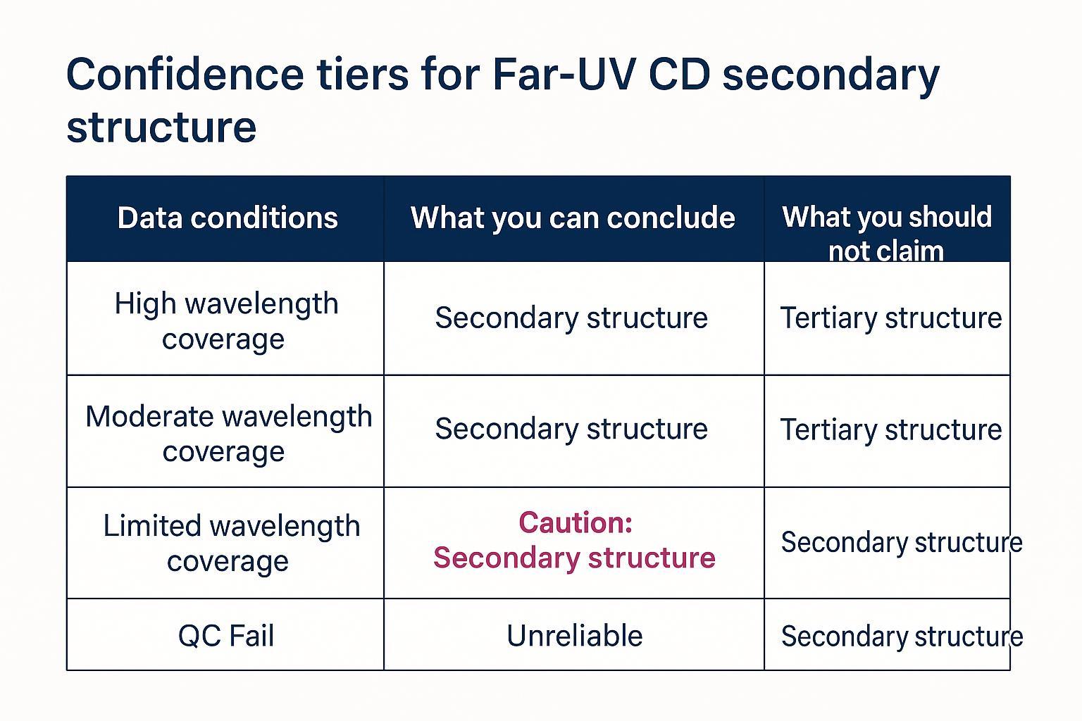
A decision boundary framework for interpreting Far-UV CD secondary structure estimates.

Aligning CD with FTIR and DSC: a practical triangulation strategy

Think of CD, FTIR, and DSC as complementary lenses:

• CD tracks secondary-structure changes sensitively, especially α-helix features near 208/222 nm and β-related signatures; it's ideal for trend screening.
• FTIR (amide I band, ~1600–1700 cm⁻¹) can sharpen β-sheet discrimination and corroborate CD, particularly when coverage is limited to 200–250 nm.
• DSC reveals thermal transitions (Tm, unfolding thermograms) and helps interpret structural stability changes.

Add FTIR/DSC when CD coverage/QC is limited, when β-sheet discrimination drives decisions, or when CD and project data disagree. For a comparison guide, see CD vs FTIR vs DSC for orthogonal confirmation.

What to request from a service provider: deliverables that make results auditable

Ask for concrete files and disclosures so you can audit assumptions and QC:

• Raw spectra (all replicates) plus matched buffer blank spectra.
• Baseline-subtracted spectra with notes on wavelength cutoff criteria.
• HT voltage and absorbance indicators vs wavelength; note any regions excluded.
• Deconvolution report: algorithms used; reference set names (e.g., SP175/SMP180); fit diagnostics (NRMSD/RMSD); overlay and residual plots; scaling/best-factor choices.
• QC summary checklist: replicate count, HT/OD ranges, baseline hygiene checks, and any deviations.
• Orthogonal recommendations (FTIR/DSC/DLS/SEC) based on confidence tier and project needs.

Practical Example (mid-body; disclosure included):

Disclosure: Pronalyse (Creative Proteomics) is our product. As a neutral example of audit-ready reporting, a Pronalyse-style deliverable set includes raw and baseline-subtracted spectra with replicate overlays, HT/absorbance logs with stated cutoffs, and a deconvolution report naming algorithms (SELCON/CONTIN/CDSSTR) and reference sets (SP175/SMP180) with NRMSD values and residuals. A QC summary flags any deviations (e.g., elevated HT below 200 nm) and labels conclusions by confidence tier (High/Moderate/Limited), recommending FTIR or DSC when β-sheet quantitation is decision-critical. If you want a feasibility check (buffer UV cutoff, pathlength, and target low wavelength), see the Far-UV CD service page: request a deconvolution report + QC summary.

Quick pre-run checklist (copy/paste)

• Confirm target coverage (ideally 190–250 nm; moderate 200–250 nm; limited >205–250 nm only for screening).
• Choose low-absorbance buffers; avoid Tris, imidazole, DTT, high salts, sugars at high concentration.
• Select pathlength to target OD ~0.9 AU at the shortest λ; verify concentration and pathlength.
• Prepare a matched buffer blank; plan 3–10 scan averages; set integration time and bandwidth.
• Control temperature and purge with nitrogen if available; monitor HT during acquisition.
• Plan deconvolution: algorithms (SELCON/CONTIN/CDSSTR), reference sets (SP175/SMP180), and fit diagnostics (NRMSD/residuals).
• Define decision boundaries: accept for screening vs require FTIR/DSC/DLS/SEC.
• For sample requirements and buffer guidance, see sample/buffer requirements (Far-UV + Near-UV).

Credibility signals:

• Method-driven guidance aligned with instrument QC and reproducibility best practices
• Transparent "what it can/can't tell you" decision boundaries to prevent over-interpretation
• Standard deliverables: deconvolution report + QC summary + replicate spectra

If you'd like a feasibility check for your sample (buffer UV cutoff, pathlength, target low wavelength) and an audit-ready deliverables plan, contact our team via the Far-UV CD service page.

By Caimei Li, Senior Scientist at Creative Proteomics. LinkedIn (Caimei Li).

Related Services

Circular Dichroism (CD) Spectroscopy Analysis Service

Far UV Circular Dichroism (CD) Spectroscopy Analysis

Near UV Circular Dichroism (CD) Spectroscopy Analysis