By Caimei Li — Senior Scientist, Creative Proteomics. Senior scientist in protein characterization with practical experience using circular dichroism (far‑UV and near‑UV) and thermal denaturation methods to assess protein higher‑order structure and stability. Connect on LinkedIn.
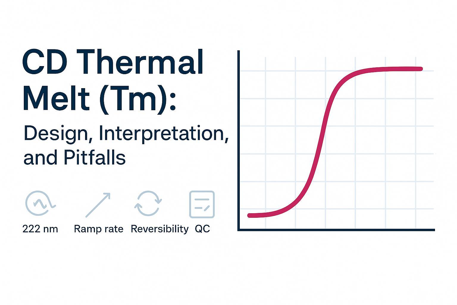
Circular dichroism thermal denaturation is a powerful way to track temperature‑driven structural change in proteins, but a CD thermal melt Tm is not a universal stability score. The midpoint you measure depends on what your chosen wavelength or spectral window "sees," on ramp rate, and on reversibility. That's why Tm ranking pitfalls happen—and why you need a disciplined workflow to avoid them.
Key takeaways
- A Tm from circular dichroism thermal denaturation reflects the monitored structural feature; it's not a one‑size‑fits‑all stability metric across mechanisms.
- Use a best‑practice SOP: define goal, pick readout (single wavelength vs spectra), select ramp rate, set a sensible temperature range, run matched blanks and replicates, check reversibility, then fit and report uncertainty.
- Stress‑test non‑equilibrium: repeat melts at two ramp rates; meaningful Tm drift signals kinetic/irreversible behavior.
- Validate wavelength choice with quick low/high‑temperature spectra; full‑spectrum series help catch baseline drift and redistribution of secondary structure.
- Watch aggregation artifacts: rising HT/noise, turbidity, or signal collapse can create pseudo‑transitions and mislead Tm ranking.
- Document defensibly: report model, wavelength(s), ramp rate, temperature range, reversibility result, fit residuals, and raw data access.
What a CD Thermal Melt Tm Can and Can't Tell You
A CD thermal melt tracks how secondary (far‑UV) or tertiary (near‑UV) structure changes with temperature. The Tm you report is the midpoint of the monitored transition, not a universal "stability" score across different unfolding pathways or irreversible systems. Multi‑domain proteins and formulation‑driven mechanism shifts can flip rankings because different conditions alter which "melting unit" the detector is sensitive to.
For scope and limits of CD signals and good practice on reporting, see the Miles & Wallace tutorial review (Chem. Soc. Rev., 2021), which details what spectral quality can and can't support and documentation expectations. Vendor and facility guides echo this caution, emphasizing reversibility and baseline management as prerequisites for thermodynamic interpretation.
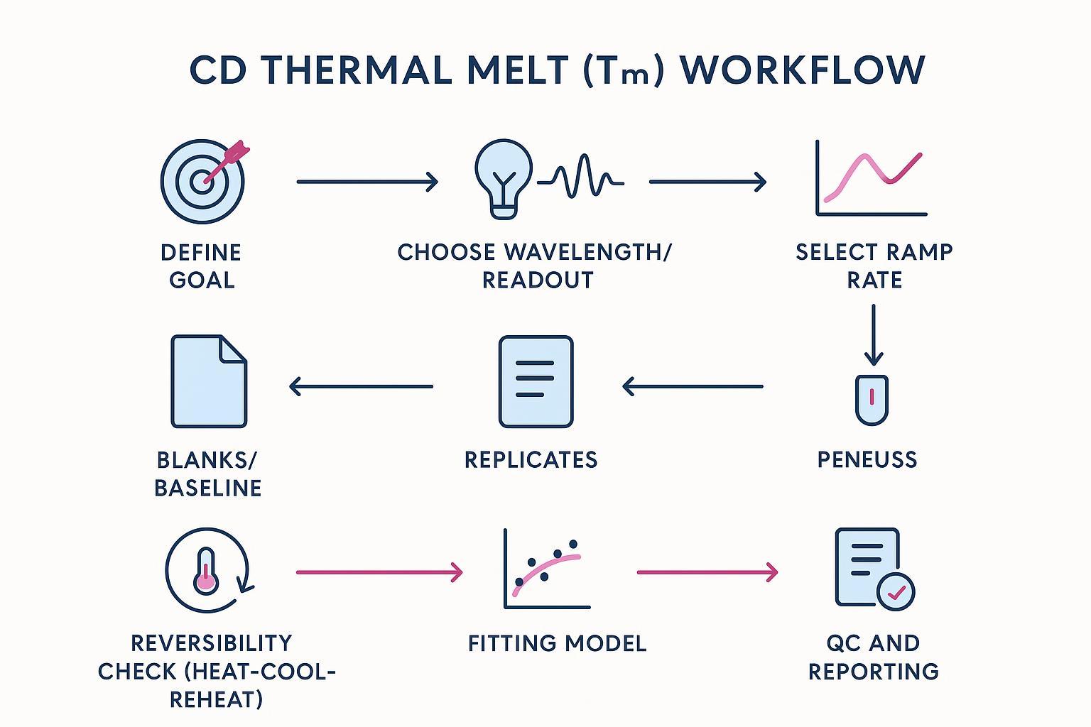
The Best‑Practice Workflow (SOP Overview)
Follow this printable protocol for reliable screening and defensible reporting.
1. Define the decision goal
- Are you screening for formulation rank ordering, or confirming mechanism? Your goal determines readout, ramp rate, and QC gates.
2. Choose the readout
- Single wavelength (fast). Use a wavelength tied to the structural feature you care about (e.g., 222 nm for α‑helix). Great for throughput when unfolding is cooperative.
- Full‑spectrum series (comprehensive). Collect spectra across temperature to verify wavelength choice, detect baseline drift, and observe secondary‑structure redistribution.
3. Select the ramp rate
- Starting point: ~1 °C/min for protein CD melts. Stress‑test at a slower rate (e.g., ~0.5 °C/min) or add short dwells near the transition to assess equilibrium. Facility primers such as Harvard's core guide Getting Started with CD and vendor notes from JASCO outline typical practice and temperature control tips.
4. Set the temperature range
- Include well‑defined pre‑ and post‑transition baselines; ensure instrument thermal stability and avoid condensation (purge below ~15 °C when relevant). The JASCO CD ebook provides practical thermal management and reversibility considerations.
5. Run matched blanks and replicates
- Acquire buffer blanks over the same temperature trajectory; target ≥3 replicates for screening to characterize variability.
6. Check reversibility (heat–cool–reheat)
- Overlay heat/cool/reheat curves or spectra. Classification determines whether thermodynamic models are valid or if "apparent Tm" is more appropriate. Core facility guides (e.g., Harvard CMI) and vendor notes (e.g., JASCO) emphasize this as the fastest high‑value check.
7. Fit and report uncertainty
- Choose two‑state vs multi‑state or apparent Tm models based on behavior; report Tm ± CI/SE, ramp rate, wavelength(s), fit residuals, and reversibility outcome. For multi‑transition or irreversible behavior, tools like CalFitter (NAR, 2018) support flexible model fitting and confidence estimation.
8. QC and documentation
- Record sample ID, concentration, buffer, cell pathlength, instrument, spectral range, wavelength(s), ramp rate, temp range, dwell times, blank method, smoothing, HT/noise flags, model, residuals, reversibility result, and raw data location.
A concise SOP like this aligns with community guidance summarized by university core facilities and vendor notes; for example, the Harvard CMI guide outlines wavelength selection and HT limits, while JASCO materials emphasize thermal control and reversibility checks.
Wavelength Choice: Single-Wavelength vs Full-Spectrum Melts
Pick wavelengths tied to the structural feature you care about, then validate with quick spectra at low and high temperature. As a practical rule: 222 nm tracks α‑helix loss; ~216 nm tracks β‑sheet features. Single‑wavelength melts are efficient for cooperative transitions, while full‑spectrum series help catch baseline drift, identify isodichroic points (supporting two‑state behavior), and reveal redistribution among secondary structures.
For background on what spectral quality can and can't support, review the Miles & Wallace tutorial which provides evidence‑based rules of CD good practice. If you need a refresher on buffer UV cutoff, pathlength, and absorbance planning before far‑UV work, see our resource center: buffer UV cutoff, pathlength, absorbance planning.
Disclosure: This guidance is provided independently of any commercial offering; cited examples and linked resources are illustrative and intended to aid experimental design, not to imply product performance, warranty, or endorsement—readers should validate methods under their own conditions before relying on results for decision-making or regulatory submissions.
Ramp Rate and Equilibration: Avoid ‘False' Tm Shifts
Ramp rate influences apparent transitions when systems are not at near‑equilibrium or are irreversible. A common starting point is ~1 °C/min with data every 1–2 °C; then repeat at ~0.5 °C/min or add 30–60 s dwells near the transition. If Tm drifts meaningfully with rate, treat the result as kinetic or apparent, not as a robust thermodynamic midpoint. Vendor brochures and facility SOPs emphasize this practice and recommend instrument stabilization and temperature calibration where available; see the JASCO CD ebook and Harvard CMI guide.
Temperature Range, Baseline Handling, and Buffer Blanks
Set baselines deliberately. Pre‑ and post‑transition segments are essential for fitting, and matched buffer blanks acquired over the same temperature path help prevent sloping baselines and pseudo‑sigmoids. Prefer UV‑transparent buffers (e.g., phosphate) for far‑UV and avoid components with strong absorbance. Manage optics: use nitrogen or dry air purge below ~15 °C to prevent condensation and bubbles; verify cell pathlength and sensor placement.
For practical planning details on buffers and cells, see our guide to sample requirements: buffer UV cutoff, pathlength, absorbance planning.
Reversibility Checks: The Fastest Way to Catch Ranking Mistakes
Run a heat–cool–reheat protocol and overlay the curves. What you see determines how to interpret Tm:
- Reversible: cooling/reheat overlays the initial curve; native spectrum recovered; thermodynamic fits supported.
- Hysteresis: cooling shows a shifted curve and partial recovery; suggests intermediates or multi‑state kinetics.
- Irreversible: no recovery on reheat; baseline drift or aggregation likely; report "apparent Tm" and avoid thermodynamic claims.
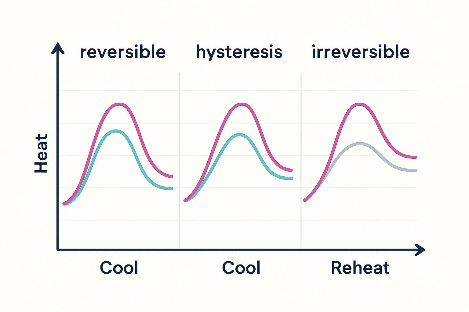
Core facility primers and vendor notes emphasize reversibility as the fastest high‑value check to prevent ranking mistakes; see the JASCO theory page for illustrative protocols.
Mid‑article CTA: Share your buffer, volume, concentration, and decision goal—we'll suggest a ramp rate and readout plan to reduce ranking errors.
Fitting Models and Reporting: Two-State, Multi-State, and Apparent Tm
Model your data according to observed behavior. Two‑state fits suit cooperative reversible unfolding and allow reporting Tm with confidence intervals and, in some cases, enthalpic parameters. Multi‑state or irreversible behavior requires more flexible models and sometimes multi‑wavelength/global analysis. When irreversibility or aggregation is present, report an "apparent Tm" and emphasize ramp rate and reversibility context alongside fit residuals.
State clearly: model used, wavelength(s) or spectral range, ramp rate, temperature range, reversibility outcome, fit residuals/NRMSD, and whether raw spectra are available for review. For advanced fitting and confidence estimation, consult CalFitter (NAR, 2018).
The Ranking Pitfalls (Why Condition A Can Look Better, Then Worse)
Ranking flips often come from:
- Baseline drift and sloping baselines (poor blank matching or thermal equilibration).
- Wavelength mis‑tracking when structure redistributes across formulations.
- Irreversible aggregation that creates pseudo‑transitions via scattering.
- Multi‑domain proteins with overlapping transitions that confound single‑wavelength melts.
Decision boundary: don't rank purely by Tm if reversibility is absent, HT/noise flags trip, baselines drift, or multi‑transition behavior is suspected. Use spectra and orthogonal methods before drawing stability conclusions.
Aggregation Artifacts: Spotting ‘Pseudo-Transitions' from Scattering
Aggregation during heating increases scattering and distorts CD signals, sometimes creating apparent sigmoids or abrupt signal collapses. Indicators include rising HT voltage, growing baseline noise, visible turbidity, the loss of isodichroic points, and poor replicate agreement. Mitigate by reducing concentration and pathlength, switching to more transparent buffers, purging optics, and adding orthogonal size readouts (DLS/SEC) to validate whether unfolding or aggregation dominates. Vendor guidance on detector high‑tension and absorbance ceilings is summarized in Applied Photophysics' HT limits note.
QC and Reproducibility: Replicates, Acceptance Gates, Documentation
Use "typical starting points," then confirm thresholds for your protein class, formulation, and instrument behavior.
- Replicates: ≥3 for screening; overlay agreement with Tm variability typically within a few degrees for practical work.
- HT/absorbance: avoid regions where instrument HT approaches vendor limits; reduce absorbance or adjust pathlength.
- Signal‑to‑noise: target robust S/N at the chosen wavelength; increase accumulations if needed.
- Baselines: matched blanks and clear pre‑/post‑transition segments; document subtraction method.
- Temperature management: purge below ~15 °C when relevant; verify in‑cell temperature where feasible.
- Documentation fields: sample ID, concentration, buffer, pathlength, instrument, ramp rate, temperature range, dwell times, wavelength(s)/spectral range, blank method, smoothing, HT/noise flags, model, residuals, reversibility result, and raw data access.
If you need a structured checklist for CD troubleshooting and quality controls, browse our resource page: CD troubleshooting and quality controls.
Troubleshooting: Noisy Curves, Drifting Baselines, Weird Shoulders, Flat Signals
| Symptom | Likely cause | Practical fix |
| Noisy curve | Absorbance/HT limit, bubbles/condensation, low concentration | Lower absorbance (buffer/pathlength), purge N2/dry air, increase accumulations |
| Drifting baseline | Blank mismatch, poor thermal equilibration | Acquire matched blanks over same temperature path; add short dwell points; stabilize instrument; verify cell temperature |
| Shoulders/multiple transitions | Multi‑domain protein or mixture | Collect full‑spectrum series; consider DSC to resolve domains; fit multi‑step models |
| Flat signal | Wavelength not sensitive to target structure, weak secondary‑structure signal | Survey spectra to choose a responsive wavelength (e.g., 222 nm for helix, ~216 nm for sheet); adjust concentration/pathlength |
When should you rerun versus switch readout? If fixes reduce noise and baselines stabilize, rerun the melt; if shoulders persist or reversibility fails, switch to full‑spectrum or add orthogonal methods before ranking.
When to Add Orthogonal Methods (and Which One)
- DSC: confirm thermal transitions, separate overlapping domains, and provide calorimetric context for ranking.
- FTIR: cross‑check changes in secondary structure (amide I/II bands) when CD is ambiguous.
- DLS/SEC: validate aggregation versus true unfolding during/after heating.
Next Step: Get a Tm Design Review and Interpretation Support
Request a Tm design review to confirm reversibility checks and aggregation risk controls before you lock the screening run. Share buffer, concentration, pathlength, volume, temperature range, and decision goal; we'll advise on ramp rate, wavelength choice, and a reversibility plan.
Explore service details and send parameters: CD spectroscopy analysis service for protein structure elucidation.
References
- Miles AJ, Janes RW, Wallace BA. Tools and methods for circular dichroism spectroscopy of proteins: a tutorial review. Chemical Society Reviews. 2021;50:8400–8417. DOI: 10.1039/D0CS00558D. (See the Royal Society of Chemistry article landing page: Chemical Society Reviews 2021 tutorial review and the PMCID mirror: PMCID PMC8328188).
- Mazurenko S, Stourac J, Kunka A, Chaloupkova R, Bednar D, Damborsky J, et al. CalFitter: a web server for analysis of protein thermal denaturation data. Nucleic Acids Research. 2018;46(W1):W344–W349. DOI: 10.1093/nar/gky358. (Canonical page at Nucleic Acids Research: NAR 2018 CalFitter web server; PubMed entry: PMID 29762722).