Quantitative Discovery Proteomics with DIA: Depth, Consistency, and Scale
What DIA Solves—and What It Requires in Return
In modern proteomics, discovery is no longer a purely exploratory endeavor. It is an engineered process—one that requires precision, reproducibility, and depth across increasingly large and complex sample cohorts. For researchers and CRO teams working in systems biology, translational studies, or biomarker discovery, these requirements translate into one central challenge:
How do you profile thousands of proteins reproducibly, without sacrificing depth or scalability?
Data-Independent Acquisition (DIA) has rapidly become the backbone of many large-scale quantitative proteomics studies. By collecting MS/MS data across all detectable peptides—rather than relying on precursor-triggered selection—DIA minimizes missing values and improves cohort consistency, even in heterogeneous or partially degraded samples such as FFPE tissues or clinical plasma.
At Creative Proteomics, we've seen DIA strategies evolve from "nice-to-have" to essential infrastructure for many discovery-driven programs. But leveraging DIA effectively requires decisions far beyond platform choice. From LC gradient design to acquisition windowing, from sample preparation to scoring strategy, every parameter can shift the outcome—and missteps accumulate quickly.
➤ See how optimized DIA sample preparation workflows minimize these missteps.
What Makes DIA Reliable for Large-Scale Discovery Proteomics
Data-Independent Acquisition fragments all ions within predefined m/z windows throughout the chromatographic peak, producing near-systematic MS/MS coverage. Compared with DDA, which relies on intensity-triggered precursors, DIA:
- Reduces stochasticity in peptide selection, dramatically lowering missingness across replicates and batches.
- Maintains consistent quantitative sampling across a cohort, which is essential for differential analysis and pathway inference.
- Trades individual-precursor purity for population-level completeness—the core bargain that supports discovery in complex matrices.
On modern Orbitrap and Q-TOF platforms—and especially with ion mobility-enabled DIA (e.g., dia-PASEF)—DIA extends into lower-abundance space without sacrificing cohort consistency. For hypothesis-free discovery across many samples, this is usually the winning move.
➤ Explore quality control strategies that ensure DIA reproducibility →
What Limits Depth in DIA—and How to Design Around It
"Depth" is not a single setting. It is the product of constraints across four layers:
- Sample layer – protein solubility, matrix suppression, abundance spread, residual contaminants.
- Separation layer – chromatographic peak capacity, dead volumes, gradient design, trap dynamics.
- Acquisition layer – window strategy, cycle time, MS2 resolution, ion accumulation, collision energy.
- Algorithm layer – feature extraction, interference modeling, retention-time (RT) alignment, FDR control, protein inference.
➤ Compare DIA data processing tools and their impact on depth and accuracy →
Your protocol is only as strong as its weakest layer. For example, chasing a 120-minute gradient with carefully crafted variable windows will not compensate for poorly controlled alkylation or salt carryover. Conversely, a modest 60-minute gradient on a healthy column and carefully tuned windows can deliver impressive depth with stable CVs.
How to Prepare DIA Samples That Withstand Scale and Complexity
Sample preparation remains one of the most underestimated sources of variability in DIA-based proteomics. To support high-throughput, discovery-grade projects—especially those involving clinical matrices, FFPE tissues, or low-yield lysates—your protocol must deliver high recovery, low background, and inter-batch reproducibility.
At Creative Proteomics, we recommend choosing sample workflows not just by efficiency, but by their tolerance to matrix type, throughput constraints, and downstream MS compatibility.
- For high-protein-load tissues and serum/plasma, S-Trap-based digestion is robust, detergent-tolerant, and compatible with both denaturing and reducing conditions. It offers consistent peptide recovery across sample lots, making it suitable for cohort studies without depletion.
- For low-input samples or automation-driven setups, SP3 bead-based cleanup provides high recovery with minimal sample loss and can be standardized in 96-well format—ideal for exosomes, cultured cells, or biopsies.
- FFPE samples demand aggressive de-crosslinking (e.g., 95°C in 2% SDS with buffer exchange), and require careful quantification post-digestion. Avoiding protein overloading is critical to prevent precipitation during alkylation or acidification.
Regardless of method, enforce strict versioning of reagents, exposure times, and buffer systems. Even minor deviations in alkylation efficiency or salt removal can lead to measurable shifts in peptide detectability and retention time.
Where possible, normalize LC-MS injection not by total protein, but by measured peptide concentration post-digestion. This compensates for matrix-specific differences in digestion efficiency and ensures consistent MS loading.
We recommend embedding a small cohort of process control samples throughout your project—pooled lysates or commercial digests—to track batch-to-batch variability. In our own QC datasets, bridging these controls has helped reduce inter-batch coefficient of variation (CV) by over 30% across studies involving plasma, CSF, and tissue homogenates.
How to Use Chromatographic Separation to Support Deeper DIA Coverage
You gain two things from better LC: peak capacity and confidence in alignment. Both feed directly into deeper, cleaner DIA identifications.
Columns & flow:
- 75 μm i.d., 25–50 cm, 1.6–1.9 μm C18 are dependable workhorses for nanoflow.
- Microflow (e.g., 1 mm i.d., 50–100 μL/min) can be attractive for robustness and throughput; expect a modest sensitivity penalty offset by excellent day-to-day stability.
Gradients:
A realistic design space for discovery is 60–120 minutes.
- ~60 min: strong for mid-sized cohorts; pair with ion mobility or carefully tuned variable windows.
- ~90 min: a pragmatic sweet spot for many tissues and non-depleted plasma.
- ~120 min: reserve for very complex matrices or when you must push depth without fractionation.
Fractionation & GPF:
- High-pH reversed-phase fractionation (6–12 fractions) is effective for building project spectral libraries without overburdening routine runs.
- >Gas-phase fractionation (GPF) builds chromatogram libraries that materially improve scoring for routine samples—especially when matrices vary slightly.
LC health monitoring:
- Inject a HeLa digest (or relevant standard) daily. Track: MS1 base peak intensity, peptide IDs, RT drift, and peak widths.
- Maintain trap and emitter; dead volumes and unstable sprays quickly erode depth and inflate CVs.

Overview of the DIA data processing and QC workflow, including retention time alignment, spectral deconvolution, MS2-based quantification, protein inference, and statistical analysis. Each step is optimized for large-scale reproducibility and biological interpretability.
Tuning DIA Acquisition Parameters for Better Quantitation and Consistency
Your design should guarantee ≥8–10 sampling points across an average peak at MS2. That single constraint guides most of the remaining choices.
Window strategy:
- Variable windows allocate narrower windows where precursors are dense (typically 400–700 m/z) and wider windows where density is sparse. This improves selectivity at no cost to cycle time.
- Overlapped windows (staggered schemes) further reduce interference but increase data and computation load—use selectively.
- For non-depleted plasma or deep tissue, window counts of 24–40 with narrower mid-m/z bins are common starting points.
Resolution & accumulation:
- On Orbitrap, pair MS2 resolution (e.g., 15k–30k at m/z 200) with IT/AGC to complete a full cycle within ~2–3 seconds.
- On Q-TOF, ensure TOF accumulation and transfer settings match your window width and expected peak width; keep the cycle ≤2 seconds for 60–90-min gradients.
Ion mobility (dia-PASEF and kin):
- Mobility adds an orthogonal dimension for interference rejection. In crowded m/z space, it pays for itself with cleaner fragment maps and better low-abundance detection.
- Use mobility-aware windowing that reuses m/z bins across mobility slices, controlling cycle time while gaining selectivity.
System suitability (pre-flight checks):
Before a batch, run SST: iRT mix, a complex digest, and blank. Verify ID counts, RT residuals, and background MS2 rates. Lock the method once SST passes; don't "tune live" mid-batch.
Spectral Libraries vs Library-Free
Three viable routes:
- Project spectral library – Build from DDA of representative samples ± high-pH fractions. Best identification rates and transferability within project scope; cost is front-loaded time.
- Chromatogram library (e.g., via GPF) – Acquire a few GPF runs per matrix/gradient; yields strong scoring for routine DIA without a full DDA campaign.
- Library-free (DirectDIA) – Fastest to start; excellent for non-model species or pilot screens; identification breadth now rivals smaller project libraries, although protein inference and PTM coverage may be more conservative.
Practical advice: if your cohort is large and the matrix is stable, a (1) project library or (2) GPF-based chromatogram library pays off across months of acquisition. If timelines are tight or species annotations are sparse, library-free is a powerful on-ramp. In all cases, version library files and keep a change log—downstream comparability depends on it.
Processing DIA Data That Yields Reproducible and Interpretable Biology
Translating DIA datasets into meaningful biological conclusions requires more than maximizing peptide or protein identifications. For discovery proteomics, the true value lies in reproducible quantitation, statistical reliability, and a clear connection between signal and biology. At Creative Proteomics, we emphasize a data strategy that integrates algorithmic rigor, study design, and QC-informed interpretation.
Aligning Retention Time and Peak Identity with Confidence
Retention time consistency is the backbone of peptide-level quantitation. DIA workflows rely on nonlinear RT alignment anchored by internal retention time (iRT) peptides or pooled bridge samples. In multi-batch designs, we recommend fixing reference runs early and applying consistent alignment thresholds across datasets. Avoid arbitrary shift-based correction, which often leads to peptide misassignment.
When using variable windows or ion mobility-enabled systems (e.g., dia-PASEF), fragment ion co-elution patterns provide another alignment layer. These should be monitored and filtered based on interference scores or extraction consistency, not just identification counts.
Quantification and Interference Management at the Peptide Level
Modern tools such as DIA-NN, Spectronaut, and EncyclopeDIA have built-in scoring models that suppress interference—but these models are only as good as the isolation strategy and window design. For dense matrices like plasma or tumor homogenates, we recommend avoiding overly wide or fixed-width windows, which increase the risk of co-fragmentation and mis-quantification.
Quantify at the peptide level using fragment ion areas. Do not aggregate to protein prematurely. For cohort-scale studies, we typically set CV acceptance thresholds at ≤20% at the peptide level, unless otherwise justified by matrix-specific challenges.
Normalization: Reference-Based Approaches Outperform Global Scaling
Total ion current normalization is often insufficient in large, heterogeneous datasets. Instead, reference sample-based normalization—using bridge samples or invariant peptides—is more robust, particularly when comparing across time, platforms, or operators.
Our internal data across >500 clinical samples show that normalization to bridge samples reduced median CVs by 25–40% compared to TIC-based methods, especially in plasma and FFPE studies.
Handling Missing Values with Statistical Discipline
Not all missingness is created equal. A peptide missing due to low abundance (MNAR) carries a different biological implication than one dropped due to random interference or extraction error (MAR).
Before imputation, filter peptides by presence thresholds (e.g., detected in ≥60% of samples in at least one group). This reduces downstream bias and improves interpretability. Avoid aggressive imputation unless justified by the specific modeling strategy (e.g., for multivariate classification).
Protein Inference: Understand the Ambiguity Before You Collapse
DIA inevitably encounters shared peptides and isoform overlap. Choose whether to report:
- Protein groups (most inclusive),
- Razor-protein assignments (most conservative), or
- Isoform-specific calls (if using annotated libraries with controlled uniqueness).
What matters is consistency and transparency. Over-aggregation may simplify figures but compromises biological interpretation—especially for post-translationally modified or closely related proteins.
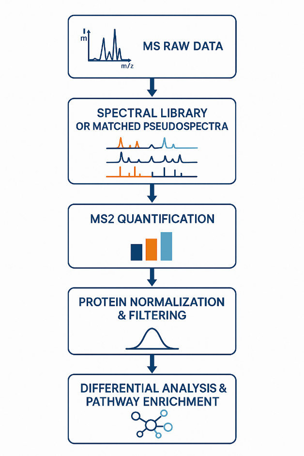
Overview of the DIA data processing and QC workflow, including retention time alignment, spectral deconvolution, MS2-based quantification, protein inference, and statistical analysis. Each step is optimized for large-scale reproducibility and biological interpretability.
Statistical Power: The Missing Link Between Quantitation and Confidence
Even with perfect alignment and normalization, your study can still fail to produce interpretable results if it's underpowered. This is one of the most frequent causes of disappointing outcomes in real-world DIA studies.
Design for power, not just coverage:
- Estimate biological variability early using pilot samples or historical data.
- Define minimum detectable fold-change relevant to your biological hypothesis (e.g., 1.5× for cytokine-level differences, 2.0× for pathway shifts).
- Randomize injection order within batches to prevent technical artifacts from masquerading as biological effects.
- Include pooled reference samples every 8–12 injections to stabilize normalization and detect drift.
We have observed in multiple CRO-scale studies that incorporating bridge samples and randomization design improved cohort-level differential expression reproducibility by >30%, even when using standard gradient lengths and window schemes.
Matrix-specific tuning that actually helps
Plasma and Serum
Non-depleted plasma presents extreme dynamic range and high protein background. Rather than introducing depletion bias, we recommend:
- Variable-width windows to avoid signal dilution in high-abundance m/z regions.
- Extended gradients (90–120 min) to improve separation of co-eluting peptides.
- Ion mobility or high-field Orbitrap platforms to increase selectivity in mid-m/z ranges.
- Bridge sample normalization, especially when matrix quality (e.g., hemolysis, lipemia) varies across cohorts.
This configuration enables >2,000 protein IDs in plasma without depletion, with CVs typically <20%.
FFPE Tissue Samples
FFPE samples are chemically crosslinked and partially degraded, making recovery and quantitation highly variable. To stabilize performance:
- Use aggressive de-crosslinking (e.g., SDS/heat), followed by complete buffer exchange.
- Quantify post-digestion peptide yields, not total protein, to avoid overloading.
- Apply library-free or GPF-based scoring, as peptide modification patterns often diverge from standard DDA-derived libraries.
- Accept more conservative protein inference, focusing on reproducibility over depth.
In our experience, bridge-sample tracking is essential for FFPE datasets, as sample age and fixation introduce batch-specific drift.
Low-Input Samples (Cells, Vesicles, Subcellular Fractions)
When starting material is limited, such as in sorted cells or EVs:
- Use SP3 or Azo-based protocols for minimal loss during lysis and cleanup.
- Normalize by peptide mass post-digestion, not estimated protein input.
- Choose shorter gradients (45–60 min) with reduced window counts to avoid signal dilution.
- When possible, aggregate technical replicates at the MS level rather than peptide-level averages.
Low-input DIA designs should favor stability and consistency over deep coverage, particularly for pathway or biomarker discovery studies.
DIA Troubleshooting Guide: How to Diagnose and Fix Performance Issues
Even optimized DIA runs can encounter signal loss, inconsistent quantification, or identification dropouts. Below is a concise reference guide to identify and resolve common problems.
Broad Peaks, Low IDs, High CVs
Cause: Column aging, trap contamination, emitter instability
Action: Replace trap/emitter; flush LC system; recalibrate injection volume based on peptide concentration
Spike in Missing Values
Cause: RT misalignment, prep variability, injection inconsistency
Action: Re-align using iRT; check gradient stability; reprocess outliers; verify injection records
Volcano Plot Artifacts or Outlier Proteins
Cause: Shared peptides, interference, over-imputation
Action: Filter for unique peptides; use project-specific library; re-analyze without imputation
Drop in MS2 Intensity or ID Count
Cause: Dirty source, unstable spray, poor ion transmission
Action: Clean ion optics; check spray voltage; validate AGC/fill time; run QC standard
Between-Batch Variability
Cause: Drift, missing bridge samples, inconsistent libraries
Action: Normalize using reference samples; fix library and FASTA versions; log all method parameters
Choosing Between DIA, DDA, and PRM: Method Selection Based on Study Goals
| Criteria | DIA (Data-Independent Acquisition) | DDA (Data-Dependent Acquisition) | PRM (Parallel Reaction Monitoring) |
| Primary Use Case | Large-scale discovery with consistent quantitation | Spectral library creation; exploratory discovery | Targeted quantitation and validation |
| Ideal Project Type | Cohort-based studies, clinical proteomics, pathway profiling | Small pilot studies, novel species, isoform/PTM exploration | Biomarker verification, focused hypothesis-driven assays |
| Quantification Strategy | Peptide-level MS2 intensity, reproducible across samples | Semi-quantitative, variable coverage | Absolute or relative, high-precision quantification |
| Missing Value Rate | Very low (deterministic sampling) | High (stochastic precursor selection) | None (targets are predefined) |
| Sample Throughput | High | Medium | Low to medium (limited targets per run) |
| Data Depth & Breadth | Broad proteome coverage with moderate ID specificity | Deeper ID potential per run but limited consistency | Focused set of known proteins |
| Reproducibility | High | Low | High |
| Use in Multi-Batch Studies | Excellent (with bridge samples & normalization) | Poor | Excellent (standard curves, spike-ins) |
| Integration Strategy | → Quantify across the full cohort | → Generate project-specific libraries | → Validate top candidates from DIA/DDA |
Frequently Asked Questions
Q1. How many proteins can DIA identify in complex samples like plasma?
In non-depleted plasma using variable-window DIA and 90–120 min gradients, >2,000 protein groups are routinely identified. Ion mobility and bridge-sample normalization further enhance depth and reproducibility.
Q2. Do I need to build a spectral library for every DIA project?
Not always.
- Use library-free DIA for pilot screens, novel species, or when time is limited.
- Build project-specific libraries when working with large, high-stakes cohorts or customized sample types.
- Consider GPF-based chromatogram libraries for improved scoring without DDA overhead.
Q3. What causes missing values in DIA, and how can I reduce them?
Most missingness comes from RT misalignment or signal interference, not true absence.
- Use stable gradients, consistent sample prep, and bridge samples.
- Avoid over-imputation; filter peptides based on presence across conditions.
Q4. Can DIA be used for post-translational modification (PTM) analysis?
Yes—with enrichment. DIA is effective for global PTM profiling (e.g., phosphorylation, acetylation) when combined with appropriate enrichment and site-level FDR control. PTM-DIA supports large-cohort quantification, but specificity is lower than PRM-based validation.
Q5. Is depletion required for plasma or serum DIA?
No. Depletion improves depth but introduces bias. Using optimized gradients, variable windows, and mobility-enhanced DIA, you can achieve excellent coverage from non-depleted plasma, especially with statistical normalization.
Q6. How do I ensure consistency across DIA batches or instruments?
- Inject pooled reference samples every 8–12 runs
- Lock gradient, library, and software versions
- Normalize at the peptide level using bridge samples
- Track system performance via ID counts, RT drift, and CV metrics
Q7. Can I combine DIA with PRM or DDA in a single project?
Yes—and you should.
- DDA for library generation
- DIA for large-cohort discovery
- PRM for targeted quantitation of key hits
References:
- Yu, Feng, et al. "Analysis of DIA proteomics data using MSFragger-DIA and FragPipe computational platform." Nature Communications 14 (2023): 39869.
- Ward, Beatriz, et al. "Deep Plasma Proteomics with Data-Independent Acquisition." Journal of Proteome Research (2024):
- Fröhlich, Katja, et al. "Data-Independent Acquisition: A Milestone and Prospect in Biomarker Screening and Discovery." Molecular & Cellular Proteomics (2024):
- Skowronek, Paul, et al. "Rapid and In-Depth Coverage of the (Phospho-)Proteome by Optimized dia-PASEF Window Placement." Molecular & Cellular Proteomics 21 (2022): e2200087.
- Martínez-Val, A., et al. "Hybrid-DIA: intelligent data acquisition integrates targeted and discovery proteomics." Nature Communications 14 (2023): 10567.
 4D Proteomics with Data-Independent Acquisition (DIA)