Ion-Mobility DIA (timsTOF) Guide: Ion Mobility, Window Design & DIA-NN Parameters
This resource serves teams evaluating Ion-Mobility DIA (aka diaPASEF) on timsTOF who want actionable settings more than theory.
What you'll get:
- How ion mobility (IM) changes DIA design and why it boosts selectivity.
- How to choose window schemes (m/z × IM) that balance coverage, precision, and duty cycle.
- A DIA-NN parameter checklist for ion-mobility DIA data (library strategy, FDR, IM-aware alignment, MBR).
- QC & release thresholds (FDR, CV, missingness, RT/IM residuals) and scenario-specific presets.
- Service-grade deliverables and reproducibility practices (parameters.json, two-matrix policy for MBR).
What Ion-Mobility DIA Adds to a DIA Service Workflow
Ion-Mobility DIA couples DIA with Parallel Accumulation–Serial Fragmentation on timsTOF. Instead of acquiring only across m/z, ion-mobility DIA slices the space in m/z × 1/K0 (ion mobility). This reduces co-fragmentation, improves interference handling, and enables narrower effective windows without exploding cycle time—if the window plan is well designed.
Service positioning:
RAW → feature extraction in m/z × 1/K0 → (library-based / library-free) search & scoring → IM/RT alignment → FDR control → MBR (if justified) → protein inference → quant matrices → QC → handoff.
Window Design for Ion-Mobility DIA — Practical Optimization
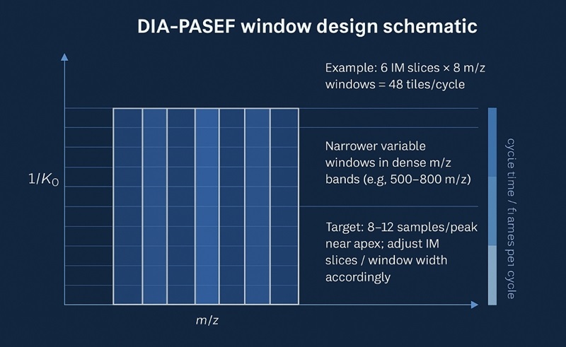
Design windows in two dimensions: m/z bands and IM (1/K0) slices. Your goal is to meet cycle-time and sampling density requirements while keeping each window's chemical complexity manageable.
Inputs that constrain your plan
- Gradient length & peak width: shorter gradients demand faster cycles (more frames per minute) to adequately sample peaks.
- Sample complexity & load: plasma/FFPE need stricter decongestion (narrower windows or more IM slices).
- Target depth & cohort size: deep coverage favors more, narrower windows; high throughput favors simpler schemes.
Choosing counts and widths (directional templates)
- IM slices (per cycle): commonly 4–8 slices give a good balance of selectivity vs. duty cycle.
- m/z windows per IM slice: typically 6–12 per slice for proteome-wide work.
- Total windows per cycle: IM slices × m/z windows (e.g., 6 IM slices × 8 m/z windows = 48 total).
- Window width: narrower at crowded m/z regions (e.g., 500–800 m/z) and/or at IM bands with higher peptide density; wider where density is low.
- Cycle time target: aim to sample chromatographic peaks 8–12× over apex; sanity-check that total windows × accumulation/ramp per frame does not violate this.
Templates (indicative, tune in pilot):
- 30 min gradient, moderate complexity: ~4–6 IM slices, 6–8 m/z windows per slice (≈24–48 total).
- 60 min gradient, standard complexity: ~6–8 IM slices, 8–10 m/z windows per slice (≈48–80 total).
- 120 min gradient, deep coverage: 8 IM slices, 10–12 m/z windows per slice (≈80–96 total).
Fixed vs. variable windows; when to use GPF
- Variable (data-density–aware) windows outperform fixed width in crowded regions.
- GPF (gas-phase fractionation) libraries: if you pursue maximum depth, schedule additional targeted windows to build a project library; otherwise pick predicted/library-free to accelerate cohorts.
Practical numbers by matrix/gradient (indicative)
| Matrix | Gradient | IM slices | m/z windows/slice | Total tiles | Notes |
| Cell/tissue | 60 min | 6–8 | 8–10 | 48–80 | Good default for cohorts |
| Depleted plasma | 60 min | 8 | 8–10 | 64–80 | Prefer narrower m/z where dense |
| FFPE | 90–120 min | 8 | 10–12 | 80–96 | Depth with conservative MBR |
Common traps (and fixes)
- Over-tiling: too many ultra-narrow tiles → cycle time inflates → under-sampled peaks. Fix: reduce IM slices or widen m/z windows until sampling ≥8×/peak.
- Uneven IM binning: one slice carries most features. Fix: re-bin 1/K0 to equalize density.
- Copy-pasting schemes across matrices: plasma ≠ lysate. Fix: for plasma/FFPE, add IM slices or narrow m/z in dense bands; increase QC frequency.
DIA-NN for ion-mobility DIA — Parameter Checklist (IM-Aware)
Use this as a pilot-to-production checklist. Record every switch in parameters.json.
Library strategy
- Library-free / predicted library for high-throughput cohorts and fast turnaround.
- Project (DDA/GPF) library for deep-coverage programs. Keep peptide candidates bounded (length 7–30 aa, 2–4 charges, enzyme specificity, ≤2 missed cleavages) to avoid false discovery inflation.
Scoring & FDR
- Set 1% peptide FDR and 1% protein FDR; disclose target–decoy method and q-value column in exports.
- Limit variable modifications (e.g., Carbamidomethyl(C) fixed; Oxidation(M) and Acetyl(Protein N-term) variable) to restrain search space.
IM-aware alignment & tolerances
- Enable IM (1/K0) in search/alignment; store IM residuals per run.
- RT alignment anchored by QC-pool; report median RT residual and 95th percentile.
- For IM residuals, define a project bound (e.g., ≤ a small fraction of your slice width) and track violations in QC.
Match-Between-Runs (MBR)
- Default to conservative MBR; use stricter evidence thresholds in plasma/FFPE.
- When MBR changes calls materially, deliver two matrices: MBR-off (primary) and MBR-on (sensitivity) for downstream robustness checks.
Cross-batch handling
- Merge batches after alignment QC passes (RT & IM).
- Normalize with a QC-anchored approach; keep a bridging QC every 10–12 injections.
- Lock export templates and grouping policy (parsimonious).
Practical compute notes
- Plan for 16–32 vCPU and 64–128 GB RAM per concurrent job (mid-tier baseline).
- Use NVMe for intermediates. Cache feature/score tables so FDR/MBR tweaks don't trigger full re-runs.
QC & Release Criteria — Measurable Thresholds and Plots
Define thresholds before production; tune them on a 10–20-injection pilot per matrix/gradient.
| Metric | Release (Pass) | Preferred Target | What to plot |
| Peptide / Protein FDR | 1% / 1% | 0.5% / 1% | FDR curves, score histograms |
| QC-pool protein CV (median) | ≤ 20% | ≤ 15% | CV distribution per QC-pool |
| Sample-level missingness | ≤ 30% | ≤ 20% | Missingness heatmap |
| RT alignment residual (median) | ≤ 30 s | ≤ 15 s | RT residuals vs. run order |
| IM alignment residual (median) | within preset bound | as low as feasible | IM residuals per run |
| MBR contribution (rows impacted) | ≤ 20% | ≤ 10% | MBR off/on delta summary |
Red/Yellow/Green gating:
- Green: all pass; proceed.
- Yellow: one marginal breach (e.g., CV ~22%); re-check normalization, continue with close monitoring.
- Red: multiple breaches or major alignment failure; hold, re-extract/re-score, or retune windows.
Outlier policy: flag samples with >2.5× MAD on missingness, RT residuals, or total intensity. Investigate carryover, spray instability, or tile congestion.
Practical Ion-Mobility DIA Configurations for Key Research Scenarios
High-throughput cohorts (budget/time sensitive)
- Windows: 4–6 IM slices × 6–8 m/z windows/slice (≈24–48 total).
- Library: library-free / predicted.
- DIA-NN: conservative MBR; QC-anchored RT/IM alignment.
- KPI direction: CV ≤ 20%, missingness ≤ 30%, stable IDs across runs.
- Why: shortest TAT with acceptable precision.
Deep-coverage discovery (ample material; depth prioritized)
- Windows: 8 IM slices × 10–12 m/z windows/slice (≈80–96 total).
- Library: project/GPF with curated filters.
- DIA-NN: strict interference control, MBR only with strong evidence.
- KPI direction: higher reproducible protein counts, lower missingness; compute cost ↑.
- Why: maximize sensitivity while maintaining auditability.
Plasma / FFPE (hard matrices)
- Windows: add IM slices or narrow m/z windows in dense regions.
- Library: predicted or project; avoid oversized candidate spaces.
- DIA-NN: raise MBR thresholds; increase QC frequency.
- KPI direction: missingness controlled; false-positive risk minimized.
- Why: chemistry-driven interference requires conservative design.
timsTOF ion-mobility DIA method migrations (cross-site or cross-batch)
- Windows: keep scheme stable across sites; only minor retuning by density.
- DIA-NN: lock versions; apply the same grouping/FDR policy.
- Deliverable: include parameters.json and export template versions.
- Why: portability and audit trails matter more than squeezing a few IDs.
Deliverables & Reproducibility (What You Receive)
- Protein & peptide matrices (.tsv) with %Missing, optional CV_QC.
- Two versions when MBR matters: MBR-off (primary) and MBR-on (sensitivity).
- Native score tables & logs + parameters.json (versions, thresholds, IM/RT alignment).
- QC bundle: FDR curves, CV distributions, missingness heatmap, IM/RT residuals.
- ID mapping (UniProt ↔ Gene Symbol ↔ Ensembl/Entrez) + field dictionary.
- Optional: container image digest (for open pipelines) to reproduce runs.
Ion-Mobility DIA Service FAQ: Windows, Libraries, QC Metrics
Q1. What's the practical advantage of Ion-Mobility DIA over conventional DIA?
A: The extra IM (1/K0) dimension reduces co-fragmentation, improving interference control and quant precision—especially in complex matrices—without blowing up cycle time when windows are well planned.
Q2. How many windows should I use for ion-mobility DIA?
A: Start with 4–6 IM slices × 6–8 m/z windows/slice for 30–60 min gradients; 8 × 10–12 for 120 min deep runs. Confirm 8–12×/peak sampling in a pilot.
Q3. Do I always need a project/GPF library?
A: No. Library-free/predicted is sufficient for many research cohorts. Build project/GPF when you need maximum depth or curated panels.
Q4. Should I enable MBR for ion-mobility DIA?
A: Use conservative MBR after alignment QC passes; disclose thresholds and deliver MBR-off/on matrices if calls change materially.
Q5. What QC thresholds should I enforce?
A: Defaults: 1%/1% FDR, QC-pool CV ≤ 20%, missingness ≤ 30%, RT median residual ≤ 30 s (preferably ≤ 15 s), and an IM residual bound aligned to your slice width.
Q6. What causes persistent RT/IM mis-alignment?
A: Column aging, temperature drift, or window congestion. Fix: re-anchor RT with QC-pool, re-bin IM slices, or widen narrow tiles in dense regions.
References:
- Meier, Florian, et al. "diaPASEF: parallel accumulation–serial fragmentation combined with data-independent acquisition." Nature Methods 17 (2020): 1229–1236.
- Meier, Florian, et al. "Online Parallel Accumulation–Serial Fragmentation (PASEF) with a Novel Trapped Ion Mobility Mass Spectrometer." Molecular & Cellular Proteomics 17 (2018): 2534–2545.
- Demichev, Vadim, et al. "DIA-NN: neural networks and interference correction enable deep proteome coverage in high throughput." Nature Methods 17 (2020): 41–44.
- Gillet, Ludovic C., et al. "Targeted data extraction of the MS/MS spectra generated by data-independent acquisition: a new concept for consistent and accurate proteome analysis." Molecular & Cellular Proteomics 11.6 (2012): O111.016717.
- Chen, Shijie, et al. "Establishing Quality Control Metrics for Large-Scale Plasma Proteomic Workflows." ACS Measurement Science Au 4.1 (2024): 32–44.
- Reiter, Lukas, et al. "Protein identification false discovery rates for very large proteomics data sets generated by tandem mass spectrometry." Molecular & Cellular Proteomics 8.11 (2009): 2405–2417. DOI: 10.1074/mcp.M900317-MCP200.
 4D Proteomics with Data-Independent Acquisition (DIA)