How to Integrate DIA Proteomics Data with Multi-Omics Platforms
Integrating data-independent acquisition (DIA) proteomics with other omics layers turns long feature lists into mechanism-level insights that matter for research decisions. This article shows, step by step, how to plan, harmonise, and model cross-layer datasets so you can move confidently from peptide intensities to pathway activity and testable hypotheses. It is written for academic groups, CRO partners, and pharma R&D teams running non-clinical, RUO projects.
Early takeaways:
- Treat study design as the first integration step.
- Standardise ID namespaces, scale, and batch handling before modelling.
- Choose a method family (feature-level, latent-space, decision-level, or network-centric) that fits your sample size, missingness, and goal.
- Validate with bridging controls, cross-validation, and stability checks, then communicate with pathway-level visuals.
➤ see our concise overview of DIA versus DDA in discovery workflows
Your search intent, our answers
"How do I merge DIA proteins with RNA-seq and metabolomics without losing signal?'
Make the data comparable first: aligned identifiers, compatible scales, thoughtful handling of missing values, and a modelling strategy that matches your cohort size and batch structure.
"What integration method fits my study design?'
Choose among feature-level, latent-space, decision-level, or network-centric approaches. The right choice depends on sample count, missing blocks, timing of assays, and whether you need discovery or discrimination.
"How do I interpret RNA–protein mismatches?'
Treat discordance as information, not error. Translation control, protein turnover, and signalling dynamics often explain the gap. Phospho-DIA clarifies when regulation happens post-translationally.
"What figures will convince reviewers and stakeholders?'
Pathway-activity heatmaps, latent-space biplots with modality loadings, enzyme–metabolite chord diagrams, and decision matrices that link your data shape to your chosen methods.
Study design is the first integration step
Cohort architecture and sampling
- Match specimens across modalities. Define one specimen ID that follows each aliquot through proteome (± phosphoproteome), transcriptome, metabolome, and lipidome.
- Choose longitudinal vs. cross-sectional early. Longitudinal designs expose trajectories; cross-sectional designs power group contrasts.
- Balance replicates by purpose. Use technical replicates to answer explicit questions (e.g., instrument drift), but invest most effort in biological replicates to stabilise integrated endpoints.
Randomisation, batch layout, and bridges
- Randomise per platform while keeping the logic isomorphic across platforms.
- Insert pooled bridge samples in every batch to quantify drift and enable batch correction.
- Pre-agree acceptance limits for ID rates, CV distributions, retention-time stability, and internal-standard behaviour (for metabolomics/lipidomics). These gates prevent "garbage in, garbage out" at integration time.
Define objectives early
- Pathway activity (not only differentially abundant proteins).
- Latent factors that summarise shared variance across layers.
- Drivers that link enzymes or kinases to metabolite shifts.
Endpoint granularity (protein groups vs. phosphosites; metabolite classes vs. species) determines mapping rules later—decide it early to avoid rework.
The DIA proteomics layer: traits that shape integration
Acquisition and quantification
DIA acquires MS/MS across predefined m/z windows, improving data completeness and cohort consistency compared with DDA. Library-based and library-free pipelines both work for integration; library-free reduces library logistics and scales well for discovery, while hybrid libraries help when deep site-level coverage matters. For signalling, pair DIA with phospho-enrichment to capture regulatory events that shift faster than protein abundance.
Quality control and normalisation
- QC that travels across layers. Track identification rate, iRT/RT stability, carryover checks, CV distributions, and proportion of quantified features per sample.
- Normalise with intent. Median, quantile, or variance-stabilising methods work; pick one that fits the intensity distribution of your dataset and stick to it.
- Treat missingness as information. DIA often exhibits MNAR behaviour near the limit of quantification. Prefer censored-value strategies or conservative imputation; avoid inventing structure below detection.
Making heterogeneous omics comparable
Identifier and ontology harmonisation
Create a robust mapping layer:
- Genes ↔ proteins: Ensembl/Gene IDs to UniProt accessions; collapse isoforms to gene level only when necessary.
- Metabolites/lipids: HMDB, KEGG, ChEBI, and LIPID MAPS with explicit adduct rules; collapse redundant adducts carefully.
- PTMs: site-specific coordinates mapped to protein sequences; maintain kinase-substrate dictionaries if pathway activity is a target.
Freeze versions of FASTA files, pathway databases, and spectral libraries. Update only by plan, not by accident.
Scale and distribution alignment
- Transform per layer (log2 or arcsinh common); z-score within layer to harmonise spread.
- Filter with restraint. Remove near-constant or poorly measured features but avoid gutting biology.
- Correct batches only when batches exist. Use bridge samples to prove technical structure before applying ComBat-style or RUV-style corrections. Over-correction is as harmful as no correction.
Choose an integration strategy that matches your constraints
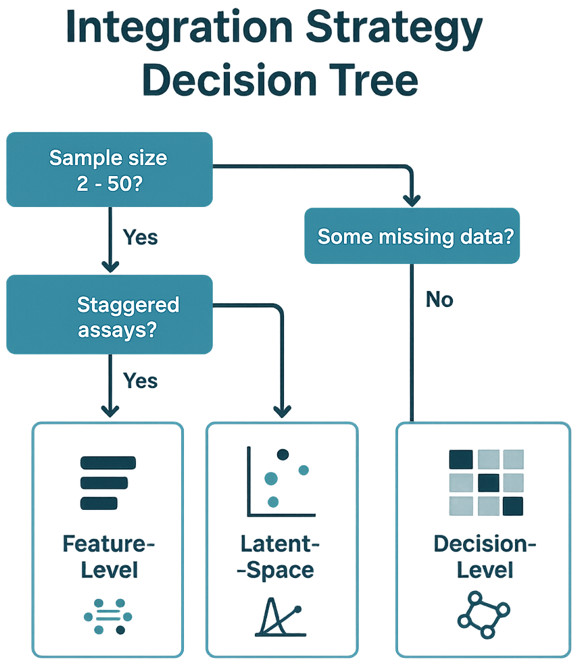
Flowchart guiding method selection based on sample size, data completeness, and study goals.
Feature-level integration: simple when data are tidy
What it is. Concatenate harmonised features, then reduce dimensionality or fit regularised models.
When to use. Matched samples, minimal missingness, moderate feature counts.
Why it helps. Fast, transparent, easy to explain.
Risks. Sensitive to noise and sparsity; can be dominated by the omics layer with the most features.
Latent-space integration: shared axes, clear stories
What it is. Multi-view factor or PLS-based models that learn components capturing shared and modality-specific variance.
When to use. Cohorts ≥ ~40 samples or smaller with strong supervision; some missing blocks tolerated.
Why it helps. Produces interpretable factors; shows which features from each modality drive separation.
Risks. Needs careful cross-validation and stability checks to avoid brittle signatures.
Decision-level integration: robust with staggered assays
What it is. Model each layer separately, then combine pathway scores, regulator activities, or per-layer predictions.
When to use. Unequal sample counts, staggered acquisition timelines, or heterogeneous QC profiles.
Why it helps. Stable, auditable, and easy to maintain; provides orthogonal replication across layers.
Risks. Slightly less granular than feature-level methods; relies on high-quality pathway maps.
Network- and pathway-centric integration: mechanism first
What it is. Build prior-knowledge graphs (PPI, enzyme–reaction, TF-target). Compute activity scores for pathways, kinases, or TFs and overlay multi-omics evidence.
When to use. Strong mechanistic priors; stakeholders want "what to test next," not only separation.
Why it helps. Converts heterogeneity into a single, human-readable layer of biology.
Risks. Depends on pathway coverage and the accuracy of prior knowledge; curate inputs carefully.
An end-to-end workflow you can run
Step 1 — Per-layer QC and normalisation
- DIA: control FDR, filter protein groups/peptides, assess CVs, lock normalisation strategy, and characterise missingness.
- RNA-seq: confirm alignment metrics, normalise counts, stabilise variance, assess unwanted variation.
- Metabolomics/lipidomics: apply internal-standard scaling, correct drift, define adduct collapsing, and verify linearity ranges.
Step 2 — Feature mapping and harmonization
Reconcile IDs to a frozen mapping table. Document one-to-many relationships (gene↔protein, metabolite synonyms) and note all merges or collapses in a manifest. Keep raw and mapped tables.
Step 3 — Confounders and batch adjustment
Build a shared design matrix: batch, run order, extraction lot, instrument, and biological covariates. Use bridges to confirm that corrections reduce technical variance without erasing signal.
Step 4 — Choose an integration method aligned to your goal
- Mechanism discovery with partial missing blocks → latent-space models.
- Discrimination with aligned samples → multi-block PLS/sparse PLS-DA.
- Staggered assays or unequal N → decision-level (pathway-score) integration.
- Prior knowledge dominates → network-centric, pathway-activity modelling.
Step 5 — Biological inference
Quantify pathway activity; assess enzyme–substrate consistency; evaluate kinase/TF activities if PTMs or transcriptional control are in scope. Interpret RNA–protein mismatches as regulatory clues rather than errors.
Step 6 — Validation and stability checks
Cross-validate latent factors and supervised components. Use permutations to check feature selection stability. Examine replicate concordance and bridge-sample behaviour. Refit models after small perturbations to test robustness.
Step 7 — Reporting and deliverables
Deliver ranked features, pathway heatmaps, integrated networks, latent-space biplots, and an executive brief that turns findings into testable, non-clinical next steps. Include containers or notebooks with parameter manifests and version-locked references.
Method selection: a quick decision matrix
| Scenario | Data shape | Primary goal | Recommended approach | Notes |
| Small cohort (<40), matched across layers | Low missingness | Discriminative signature | Multi-block PLS / sparse PLS-DA | Keep features parsimonious; strong cross-validation. |
| Moderate cohort (≥40), some missing blocks | Exploration | Shared vs. specific drivers | Multi-omics factor model | Robust to block-missing; interpretable loadings. |
| Unequal sample counts or staggered timelines | Heterogeneous | Stable, auditable decisions | Decision-level (pathway scores) | Align by pathway; easy to explain and maintain. |
| Strong mechanistic prior (enzymes↔metabolites; kinases↔substrates) | Any | Mechanism and intervention points | Network-/pathway-centric | Best for communicating causality. |
From proteins to mechanisms: interpreting cross-layer evidence
RNA–protein discordance is information
mRNA and protein changes often diverge due to translation control, protein turnover, or compartmentalisation. Treat mismatches as hypothesis generators. For example, flat RNA with rising protein can suggest increased translation or stabilisation; rising RNA with flat protein may imply fast turnover or downstream bottlenecks. Add phospho-DIA to test whether signalling explains the mismatch.
Enzyme–metabolite consistency
Ask three questions on every pathway:
- Do enzyme abundance or phosphorylation changes support the observed metabolite ratios?
- Are changes consistent with thermodynamic direction and cofactor status?
- Could bypass routes or compartmentation explain exceptions?
When patterns disagree, propose flux redistribution or post-translational control as follow-up experiments.
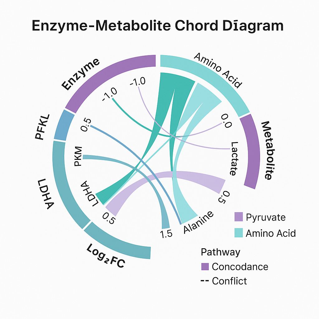
Cross-Omics Enzyme–Metabolite Chord Diagram
Visual comparison of protein (left) and metabolite (right) fold changes within a shared pathway. Colored chords highlight consistent or divergent shifts.
Common pitfalls and how to avoid them
ID Mismatch Across Datasets
Problem: Gene, protein, and metabolite IDs often don't align.
Risk: Key features get lost or misassigned.
Fix: Use consistent, version-locked ID mappings; document all conversions; test mapping on a subset before scaling.
Blind Imputation of Missing Values
Problem: Missing values in proteomics are often due to low abundance—not random loss.
Risk: Improper imputation distorts patterns and inflates false positives.
Fix: Understand the missingness pattern first. Use conservative or censored models—or leave missing values untouched if the method allows.
Batch Correction Without Evidence
Problem: Batch correction is often applied without verifying if batch effects exist.
Risk: You may remove true biological signals.
Fix: Confirm batch structure using bridge samples. Always check before/after variance plots.
Overfitting with Small Sample Sizes
Problem: Complex models need sufficient data.
Risk: Small or noisy datasets lead to unstable or misleading results.
Fix: Use simpler, robust methods (like decision-level integration) for small cohorts; prioritise data quality over model complexity.
Ignoring PTMs When They Matter
Problem: Some biological processes are regulated by modifications, not abundance.
Risk: Total protein data alone may miss critical signals.
Fix: Include phospho-DIA or PTM layers when studying signalling or stress response.
Deliverables Don't Match Project Goals
Problem: You get long feature tables, but no clear biological conclusions.
Risk: Time is wasted translating results into decisions.
Fix: Define expected outputs early—pathway scores, key drivers, or network views. Request versioned reports and ready-to-use figures.
Case studies from the literature (research-use only)
Case Study 1 — Feeding time shapes liver pathways via multi-omics coordination
Design. A mouse liver study comparing feeding schedules combined proteomics, lipidomics, transcriptomics, and metabolite measurements to probe circadian control.
Integration. Factor/component approaches summarised shared axes that tracked meal timing. The integrated factors connected protein and lipid cycles with transcriptional rhythms.
Outcome. The study identified convergent pathways regulating hepatic metabolism under distinct feeding regimes. The cross-layer agreement strengthened the mechanistic narrative.
Reference. Huang, R., et al. Nature Communications (2023). DOI: https://doi.org/10.1038/s41467-023-41759-9
Case Study 2 —Library-based DIA phosphoproteomics enables pathway-level discovery
Design. Large-scale phosphoproteomics using DIA with hybrid libraries enabled dense site-level quantification under defined signalling stimuli.
Integration. Phosphosite changes were combined with prior kinase–substrate knowledge and, where available, transcript measurements to infer regulator activities.
Outcome. The integrated analysis produced robust pathway activity calls, showing the value of DIA for signalling-centric multi-omics.
Reference. Kitata, R. B., et al. Nature Communications (2021). DOI: https://doi.org/10.1038/s41467-021-22759-z
Case Study 3 — Latent-space integration at scale with MOFA+
Design. MOFA+ provided a general framework for integrating multiple modalities with missing blocks and complex group structures.
Integration. The method separated shared variance from modality-specific effects, making factor interpretation straightforward and robust.
Outcome. For exploration-first projects and staggered assays, MOFA+ offers a stable entry point to multi-omics hypothesis generation.
Reference. Argelaguet, R., et al. Genome Biology (2020). DOI: https://doi.org/10.1186/s13059-020-02015-1
Case Study 4 — Supervised multi-omics signatures with DIABLO
Design. DIABLO (multi-block PLS) learns sparse, coordinated signatures across omics layers for phenotype discrimination.
Integration. The framework selects minimal sets of features from each modality that move together, aiding interpretation and downstream validation.
Outcome. When the goal is a compact, interpretable panel rather than broad exploration, DIABLO excels with rigorous cross-validation.
Reference. Rohart, F., et al. PLOS Computational Biology (2017). DOI: https://doi.org/10.1371/journal.pcbi.1005752
What you will receive in a well-run integration project
- Study-design consultation that aligns layers, sampling, and bridging plans to your research question.
- DIA data package with protein/peptide/phosphosite tables, QC metrics, missingness audits, and normalisation rationale.
- Harmonised matrices: frozen ID mappings, scale alignment, and batch-adjusted tables ready for modelling.
- Integration models: latent-space factors or decision-level pathway scores with cross-validation and stability diagnostics.
- Executive brief: a short, decision-oriented summary translating findings into next experiments (strictly research-use)
Frequently asked questions
Can I integrate DIA proteomics with single-cell RNA-seq data?
Yes. Aggregate single-cell data into pseudobulk profiles by condition or cluster. Then align sample IDs with your DIA dataset. For true single-cell resolution, use the pseudobulk trends to annotate downstream cell-level interpretations.
What is the minimum sample size for reliable multi-omics integration?
For unsupervised models like MOFA+, at least 40 samples are recommended. For supervised methods (e.g., DIABLO), you can go lower, but only with strong cross-validation. Fewer samples? Consider decision-level integration instead of feature-level fusion.
What if different omics datasets were generated at different times?
Use decision-level integration. Compare pathway scores or driver activities instead of raw features. Bridge samples can help you assess consistency across acquisition windows.
How do I combine phosphoproteomics with total protein data?
Use phospho-DIA to capture regulatory events and total protein to provide abundance context. Then infer pathway or kinase activity by combining both layers. Avoid interpreting phospho changes without normalisation to total protein levels.
References:
- Huang, R., et al. Multi-omics profiling reveals rhythmic liver function shaped by meal timing. Nature Communications 14, 6086 (2023). DOI: 10.1038/s41467-023-41759-9.
- Kitata, R. B., et al. A data-independent acquisition-based global phosphoproteomics system enables deep profiling. Nature Communications 12, 2539 (2021). DOI: 10.1038/s41467-021-22759-z.
- Argelaguet, R., et al. MOFA+: a statistical framework for comprehensive integration of multi-modal single-cell data. Genome Biology 21, 111 (2020). DOI: 10.1186/s13059-020-02015-1.
- Rohart, F., et al. mixOmics: An R package for "omics feature selection and multiple data integration. PLOS Computational Biology 13(11): e1005752 (2017). DOI: 10.1371/journal.pcbi.1005752.
- Singh, A., et al. DIABLO: an integrative approach for identifying key molecular drivers from multi-omics assays. Bioinformatics 35(17): 3055–3062 (2019). DOI: 10.1093/bioinformatics/bty1054.
- Bekker-Jensen, D. B., et al. Rapid and site-specific deep phosphoproteome profiling by data-independent acquisition. Nature Communications 11, 787 (2020). DOI: 10.1038/s41467-020-14609-1.
- Graw, S., et al. Multi-omics data integration considerations and study design for systems biology. Molecular Omics 17(2): 170–185 (2021). DOI: 10.1039/d0mo00041h.
 4D Proteomics with Data-Independent Acquisition (DIA)