



Introduction
The Physics of the Separation: The Van Deemter Equation
Stationary Phase Selectivity and Column Physics
Injection Physics and Sample Volatilization
Detection Physics: GC-MS Coupling and the Meaning of Structural Signal
GC-FID vs GC-MS: Choosing the Detector by Analytical Intent
A Practical Method-Development Sequence for Precision GC
Conclusion
FAQ
Related Services
Introduction
Gas chromatography is often introduced as a technique for separating volatile compounds. That description is correct, but it is too broad for serious method development. In real analytical work, GC performance depends on four linked controls: transport physics, stationary-phase chemistry, inlet transfer, and detector behavior. When a method underperforms, the problem is rarely that GC is the wrong platform. More often, the method is operating at the wrong linear velocity, using a phase with the wrong selectivity, relying on a film thickness that does not fit the volatility window, or losing band quality in the inlet before separation even starts.
This is why precision GC should not be framed as a generic overview of injectors, columns, ovens, and detectors. Those parts matter, but they do not explain why one method delivers sharp, well-spaced, decision-grade peaks while another produces overlap, drift, discrimination, or unstable identification confidence. The real questions are more demanding. What sets the efficiency ceiling of a GC run? What actually determines whether two compounds move apart? Why do early volatile peaks fail so easily in poorly designed methods? And when does a workflow need GC-MS rather than GC-FID?
These questions matter most in projects where chromatographic quality has downstream consequences. In untargeted metabolomics, poor separation does not just broaden peaks. It weakens annotation confidence and complicates feature curation. In short-chain fatty acid analysis, weak front-end retention can compromise the very analytes the study is trying to measure. In xenobiotic metabolites analysis, unstable inlet transfer can turn a reproducible method into a noisy one with false uncertainty. In all of these cases, GC is not just a separation tool. It is a controlled physical system whose settings shape the quality of the final biological or chemical conclusion.
The same logic applies when GC sits inside a broader analytical offering. In a full metabolomics service, the chromatogram is not the endpoint. It is the foundation for identification, statistical comparison, and biological interpretation. If the front end of the method is weak, every later stage becomes more difficult. That is also why GC design choices matter in targeted metabolomics, where retention stability, analyte recovery, and interference control often matter just as much as detector sensitivity.
The right starting point, then, is not a hardware tour. It is the physics of plate height.
The Physics of the Separation: The Van Deemter Equation
At the center of chromatographic efficiency is the relationship between plate height and carrier-gas velocity. In capillary GC, that relationship is usually written as:
[H = A + B/u + C · u]
Here, (H) is the height equivalent to a theoretical plate, and (u) is the linear velocity of the carrier gas. Lower (H) means better efficiency. That one statement carries most of the practical meaning of the equation. It explains why both very slow and very fast conditions can damage a separation, even when the same column and temperature program are used.
What the equation means in practice
The first term, A, is typically described as eddy diffusion. In packed columns, this term reflects the fact that molecules can follow different paths through the particle bed. In capillary GC, that contribution is much smaller because the gas moves through an open tube rather than through a packed maze. So although the A term remains part of the classical framework, it is usually not the dominant reason a capillary method loses performance.
The second term, B/u, describes longitudinal diffusion. This is the low-velocity penalty. When carrier-gas flow is too slow, analytes remain in the column too long. During that extra residence time, the band diffuses along the direction of travel. The peak spreads before it ever reaches the detector. The method becomes slower, but not necessarily better. In fact, it often becomes less efficient.
The third term, C·u, describes mass-transfer resistance. This is the high-velocity penalty. When the gas moves too quickly, analytes do not have enough time to equilibrate between the mobile phase and the stationary phase. Some molecules are still interacting with the stationary film while others have already re-entered the gas stream. The band loses coherence. Peaks broaden, and closely eluting compounds begin to collapse into each other.
The practical meaning is clear:
- At low linear velocity, diffusion becomes the main source of band broadening.
- At high linear velocity, incomplete equilibration becomes the main source of band broadening.
- Between those extremes lies an operating zone where the system reaches its best efficiency.
That middle region is the real kinetic sweet spot of the method. It is not a theoretical curiosity. It is one of the most important controls in day-to-day GC performance.
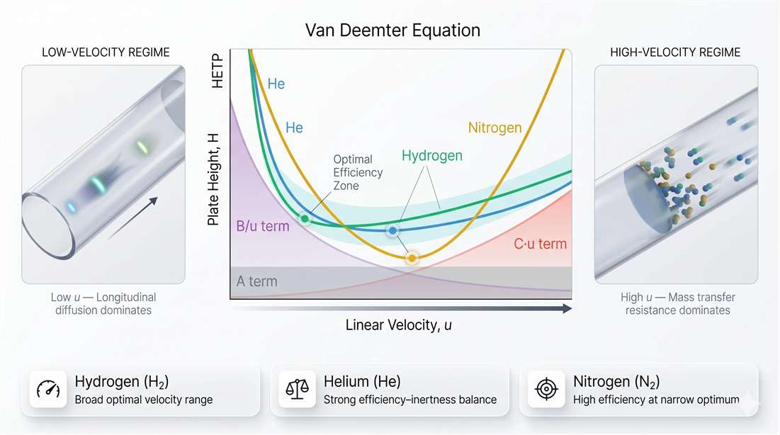
Figure 1. Van Deemter curve and the operational sweet spot for capillary GC. A comparative view of hydrogen, helium, and nitrogen illustrates how chromatographic efficiency changes with linear velocity. At low velocity, longitudinal diffusion increases band spreading. At high velocity, mass-transfer resistance becomes the dominant penalty. The most useful operating zone sits between these extremes.
Why carrier gas changes the method
Carrier gas is not just a supply choice. It changes how forgiving the method will be. Hydrogen, helium, and nitrogen behave differently because their diffusion characteristics differ. That changes where the efficiency minimum appears and how broad the usable velocity window becomes.
In practical terms, hydrogen usually supports faster operation without a sharp collapse in efficiency. Helium often provides a strong balance between performance and chemical inertness. Nitrogen can produce high efficiency near its optimum point, but that optimum is narrower. Once the method is pushed too fast, performance tends to fall off more sharply.
This matters because few analytical methods operate under perfectly static conditions. Throughput pressure is common. Sample complexity shifts. Columns age. Minor changes in flow control or instrument condition can move the system away from its best point. A carrier gas with a broader useful operating range gives the method more tolerance. That can be valuable in volatile impurity work, higher-throughput screening, and discovery pipelines where speed matters but resolution cannot be sacrificed casually.
This is especially relevant when GC data must support downstream interpretation rather than stand alone. In GC-MS/MS untargeted metabolomics, a method that runs fast but sacrifices separation can create more feature ambiguity, not more productivity. In unknown metabolite identification, weak peak separation can make later spectral interpretation look harder than it should be.
From plate height to resolution
It is tempting to think that efficiency is the whole story. It is not. A method can be efficient and still fail to separate the compounds that matter. Lower plate height gives narrower peaks. Narrower peaks improve resolving power. But actual resolution also depends on retention and selectivity.
That is why flow optimization alone rarely rescues a difficult separation. It can improve peak shape, but if the stationary phase is not creating the right interaction differences, the analytes may still elute too close together. Good GC method development therefore separates two questions:
- How efficiently can the system move a band?
- How selectively does the phase distinguish one analyte from another?
The first question is kinetic. The second is thermodynamic. Both have to be right if the chromatogram is expected to support confident decisions.
What wrong velocity looks like
When linear velocity is too low, the chromatogram often shows long run times and broader peaks than expected, especially later in the run. The method feels gentle, but the band has had too much time to diffuse.
When velocity is too high, the method may appear attractive because it is fast, but critical pairs begin to collapse. The chromatogram can still look visually acceptable at a glance, which is why this failure mode is often missed. The problem is not always ugly peak shape. The problem is that the peaks no longer separate enough to support reliable integration or identification.
This becomes even more important when film thickness is high, because analytes need more time to move in and out of the stationary phase. That link between linear velocity and stationary-phase transfer is the bridge to the next part of the method: selectivity and column physics.
Stationary Phase Selectivity and Column Physics
If the Van Deemter equation tells us how well a band can travel through the column, the stationary phase tells us whether that band should separate from its neighbors at all. This is why phase selection sits at the center of serious GC method development. Column length, internal diameter, and flow all matter. But if the phase chemistry is wrong, the method starts from a weak position.
Why "polar vs nonpolar" is too simple
Many introductory GC discussions explain column choice using a simple polarity rule. That rule is useful, but it is only the surface layer. In real separations, retention depends on specific interaction patterns between analytes and the stationary phase. These can include dispersion-driven interactions, dipole-related interactions, proton-sharing effects, and hydrogen-bond-associated behavior.
That is why two compounds with similar boiling points can separate very differently on two different phases. Their bulk volatility may be similar, but their interaction strengths with the stationary film are not.
So the better method-development question is not "Is my sample polar?" The better question is "What interaction differences do I need the phase to amplify?" That shift matters because a method does not need the most retentive phase. It needs the phase that changes peak spacing in the most useful way.
McReynolds constants and practical selectivity logic
McReynolds constants are helpful because they move column selection beyond vague descriptors. They compare how probe compounds behave on a given phase relative to a nonpolar reference. In practical use, this helps analysts think more precisely about which interaction tendencies a phase emphasizes.
The real value is not in memorizing numbers. The value is in the mindset. A stationary phase is not a single scale from "less polar" to "more polar." It is a selective environment with preferences. Those preferences determine which compounds move apart and which remain crowded together.
This becomes especially important in chemically broad sample sets. In a tightly defined targeted method, the interference pattern may already be known. In discovery-style workflows such as untargeted metabolomics or metabolomics service, the method must behave sensibly across multiple classes of compounds. That demands more than generic polarity matching. It demands an interaction-aware column strategy.
The same requirement appears in lipid-related volatile analysis. In fatty acids metabolomics service and total fatty acids analysis, selectivity decisions are rarely just about retention. They are about separating related species cleanly enough that downstream quantitation and biological interpretation remain credible.
Film thickness is a major variable, not a minor one
Film thickness, written as (d_f), is often treated like a secondary tuning parameter. In practice, it changes the behavior of the entire chromatogram.
A thicker film gives analytes more stationary-phase volume to partition into. That usually increases retention, especially for highly volatile compounds. It also increases phase capacity. This can help prevent overload at the front of the run and improve the interpretability of early peaks.
But the gain is not free. A thicker film also increases the time required for analytes to move in and out of the stationary phase. That raises the stationary-phase contribution to mass-transfer resistance. Under faster conditions, that penalty becomes easier to see. Peaks broaden. Speed becomes less forgiving. A method that looks improved at the front end may become less efficient elsewhere.
This is why film thickness should always be treated as a strategic variable. It affects:
- retention strength
- phase capacity
- front-end peak spacing
- tolerance to volatile overload
- mass-transfer burden during fast analysis
A thick film is not automatically better. A thin film is not automatically faster in a useful sense. Each one solves a different problem.
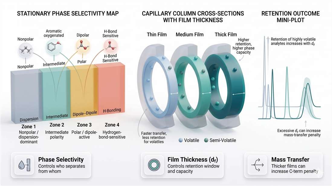
Figure 2. Stationary phase selectivity and film thickness as dual controls of GC behavior. Stationary-phase chemistry defines the interaction profile of the method. Film thickness then modifies retention strength, analyte capacity, and mass-transfer burden. Thick films can improve retention of highly volatile compounds, but they also increase the risk of peak broadening when transfer becomes diffusion-limited.
Highly volatile versus semi-volatile compounds
This is where (d_f) becomes especially important. If the method targets highly volatile analytes, a thin film may not hold them long enough. They can elute too close to the dead time, with weak spacing and poor robustness. In such cases, a thicker film often improves the usable front end of the chromatogram.
For semi-volatile compounds, the situation is different. Retention is often already adequate. Increasing film thickness may add little useful selectivity while increasing run time and broadening. The method becomes slower without necessarily becoming better.
That is why broad-boiling-range methods are difficult. The same film thickness that helps the first few peaks may compromise the later ones. Good method development is not about optimizing for the average analyte. It is about deciding which part of the volatility range requires the most control.
This tradeoff matters in real service workflows. In organic acid analysis, front-end retention and derivatized-analyte behavior often determine whether early compounds are quantifiable. In biogenic amine analysis solution, sample chemistry and transfer behavior can place different demands on retention and peak shape. The method has to be built around the hardest region of the chromatogram, not the easiest one.
How to think about phase and film together
One of the most common mistakes is to choose phase chemistry first and then treat film thickness as a convenience setting. The better approach is to think of them as a coupled system:
- Phase chemistry determines who separates from whom.
- Film thickness determines how strongly volatile compounds are retained and how much transfer burden the method can tolerate.
If a method is failing at the front of the run, phase chemistry alone may not solve it. The analytes may simply not be spending enough time in the stationary phase. If a method is broad and sluggish, more retention may not help. The system may already be paying too much mass-transfer penalty.
Kovats retention index: beyond raw retention time
Retention time is useful inside a single run. It is much less useful as a transferable identity coordinate across methods, systems, or laboratories. This is why the Kovats retention index remains so powerful.
The logic is straightforward. Instead of describing an analyte only by its observed retention time, the method places that analyte relative to adjacent n-alkane standards. That converts raw elution position into an indexed coordinate. The result is more portable than retention time alone and more useful when retention behavior needs to support identification.
This does not make retention behavior universal. Phase chemistry and method conditions still matter. But it does make retention information more stable and more interpretable across contexts.
In unknown-rich workflows, this is a major advantage. A spectral library hit can look plausible even when it is wrong. If the retention index is inconsistent with the proposed identity, confidence should drop. If both the spectral pattern and the retention index support the same structure, the annotation becomes much stronger.
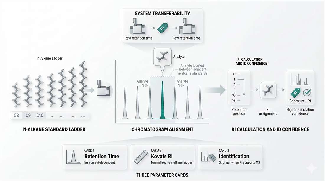
Figure 3. Kovats retention index workflow for transferable identification. An analyte is positioned between adjacent n-alkane standards, converting raw retention into an indexed coordinate. This indexed value is more portable than retention time alone and becomes especially valuable when combined with mass spectral evidence for unknown identification.
Why retention index matters in advanced workflows
For MOFU and BOFU readers, retention index is not just a technical detail. It signals analytical maturity. It shows that the method is designed for confirmation, not just detection.
In untargeted studies, isomer-rich panels, and cross-batch comparison workflows, spectrum-only identification can be too weak. Retention index adds an orthogonal layer of support. It helps answer a more rigorous question: not just whether the proposed match is spectrally plausible, but whether it is chromatographically plausible as well.
That is exactly the kind of logic advanced buyers look for when evaluating a platform or partner for volatile analysis, metabolomics, or unknown compound identification. It also connects naturally to downstream bioinformatics for metabolomics and multivariate analysis service, because feature annotation quality strongly affects everything that happens after peak picking.
Injection Physics and Sample Volatilization
Many GC problems are blamed on the column because the separation happens there visibly. In practice, the failure often begins earlier. If the sample does not enter the column as a narrow, well-controlled band, the column is being asked to repair a problem it did not create.
That is why inlet physics deserves more attention than it usually gets. Split ratio, liner volume, solvent expansion, pressure conditions, and thermal discrimination are not secondary details. They are first-stage controls of chromatographic quality.
Split and splitless are transfer strategies
Split and splitless injection are often taught as operating modes. That is correct, but incomplete. They are better understood as transfer strategies.
In split injection, only part of the vaporized sample enters the column. The rest exits through the split vent. This is useful for concentrated samples because it protects the column and detector from overload while helping preserve peak shape.
In splitless injection, most of the analyte is directed toward the column during the transfer window. This is why splitless mode is preferred for trace analysis. The goal is maximum analyte delivery, not dilution.
The important point is that choosing split or splitless is only part of the solution. Successful transfer also depends on how the sample volatilizes inside the liner, how the vapor cloud behaves under inlet temperature and pressure, and whether the analyte band stays compact as it moves toward the column entrance.
This distinction is easy to underestimate in commercial settings. In targeted metabolomics, trace-level accuracy can be limited as much by transfer quality as by detector response. In short-chain fatty acid analysis, early-eluting compounds are especially sensitive to poor inlet control because there is so little chromatographic margin for recovery once the band shape has already been damaged.
Vapor expansion and the backflash problem
One of the most important inlet failures is backflash. This occurs when the injected solvent expands into a vapor volume larger than the liner can safely contain.
When that happens, the vapor cloud no longer stays inside the intended transfer path. Part of it moves into regions of the inlet that were never meant to support controlled sample transport. Some analyte may condense. Some may adsorb. Some may re-enter the system inconsistently. The result is often a combination of poor reproducibility, distorted peaks, memory effects, and unexplained analyte loss.
Backflash is not a mysterious contamination issue. It is a physical volume mismatch.
That is why solvent expansion should be treated as a design parameter. Before changing columns or temperature programs, the method should answer a simpler question: can the solvent vapor cloud fit inside the liner under the actual inlet conditions? If the answer is no, downstream optimization will never be fully reliable.
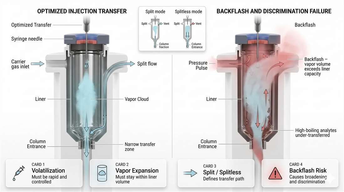
Figure 4. Injection physics in GC: optimized transfer versus backflash failure. A well-matched inlet keeps the vaporized sample inside the liner and transfers a narrow band toward the column entrance. A poorly matched inlet allows the vapor cloud to exceed liner capacity, producing backflash, broader transfer, carryover risk, and unstable reproducibility.
Thermal discrimination and heavy-end loss
Backflash is not the only inlet failure. Some methods fail more selectively. High-boiling analytes are especially vulnerable to incomplete volatilization and transfer bias.
If inlet heating, liner geometry, or vapor routing are not well matched to the sample, lighter compounds may transfer efficiently while heavier compounds lag behind or become under-represented. The chromatogram then looks artificially strong at the early and middle part of the run while the upper-boiling region is suppressed.
This is dangerous because the method can still look acceptable at first glance. Early peaks are sharp. Replicates may appear stable. But the method is biased against the compounds that are hardest to transfer.
That is why inlet optimization should never be judged only by the first few analytes. It should be judged across the full boiling-range window of the method. This point is especially relevant in fatty acids metabolomics service and organic acid analysis, where apparent front-end success can hide selective losses elsewhere in the profile.
Why inlet control matters for serious analytical work
For advanced buyers and method developers, this section is more than troubleshooting advice. It is a marker of technical depth. A credible GC workflow is not defined only by instrument ownership. It is defined by control of the transfer process.
That matters in trace analysis, volatile metabolite profiling, unknown screening, and any project where repeatability and structural confidence are important. A workflow that ignores vapor expansion, liner behavior, and discrimination risk may still generate peaks, but it will struggle to generate trust. That is one reason clients evaluating broader packages such as integrated proteomics and metabolomics analysis or integrated metabolomics and microbiomics analysis increasingly care about front-end analytical control, not just downstream data volume.
Detection Physics: GC-MS Coupling and the Meaning of Structural Signal
Once the column has done its job, the next question is no longer just whether peaks are separated. The question becomes more demanding: what kind of evidence does the detector return, and is that evidence strong enough for the analytical goal?
This is where many GC articles stay too shallow. They usually say GC-FID is good for quantitation and GC-MS is good for identification. That is true, but it is not enough for method planning. For MOFU and BOFU readers, detector choice is not a feature checklist. It is a decision about what kind of proof the workflow must deliver.
If the task is routine quantitation of a known analyte class, a stable carbon-responsive detector may be the best answer. If the task is unknown identification, structural confirmation, or interpretation in a complex matrix, the detector has to do more. It has to return identity-rich signal, not just peak area.
That is why GC-MS coupling matters. It turns chromatographic separation into a structurally interpretable workflow. The column narrows the chemical space. The ion source and mass analyzer then determine how much of that chemical space becomes usable analytical evidence.
Electron ionization and why 70 eV still matters
Electron ionization, or EI, remains the default ionization mode in GC-MS for a reason. It is energetic, reproducible, and rich in fragmentation. At the standard 70 eV setting, gas-phase molecules are bombarded by electrons and converted into radical cations that often break into highly characteristic fragments.
That fragmentation is the strength of EI. It creates a spectral pattern that behaves like a fingerprint. For many analytes, especially in environmental, food, toxicology, and metabolomics workflows, that fingerprint can be matched against reference libraries with strong practical value.
This is why EI remains central to unknown screening. The analyst is not only asking whether a peak exists. The analyst is asking whether the fragment pattern supports a specific structure strongly enough to distinguish it from close alternatives.
But EI also has a limitation. Because it is energetic, the molecular ion may be weak or missing. That can make molecular-weight confirmation harder, especially for labile compounds or analytes that fragment too efficiently. In those cases, the spectrum is rich, but parent-level confidence is weaker than the analyst would like.
This tradeoff matters directly in unknown metabolite identification, where rich fragmentation can accelerate library-style annotation, but parent-ion uncertainty may still keep the final call from becoming fully convincing.
Chemical ionization and when softer signal is better signal
Chemical ionization, or CI, solves a different problem. Instead of letting direct high-energy electron impact dominate the event, a reagent gas is ionized first, and the analyte is then ionized through ion–molecule reactions. The process is gentler. Fragmentation is reduced. Molecular-ion or quasi-molecular-ion information is more likely to survive.
That changes the meaning of the spectrum. CI usually does not generate the same fingerprint richness as EI. But it often does a much better job preserving molecular-mass evidence. When EI gives a spectrum full of useful fragments but no convincing parent signal, CI can provide the missing anchor.
So the real decision is not "EI or CI is better." The real decision is what kind of uncertainty still needs to be reduced.
- If the main uncertainty is structural pattern matching, EI is often the better choice.
- If the main uncertainty is molecular weight or parent-ion confirmation, CI often adds more value.
- If the sample is complex and the identity stakes are high, EI and CI may be best used as complementary modes.
This becomes especially important in GC-MS/MS untargeted metabolomics, where annotation often depends on more than one layer of evidence, and in xenobiotic metabolites analysis, where structurally related compounds can remain ambiguous if parent-level confirmation is weak.
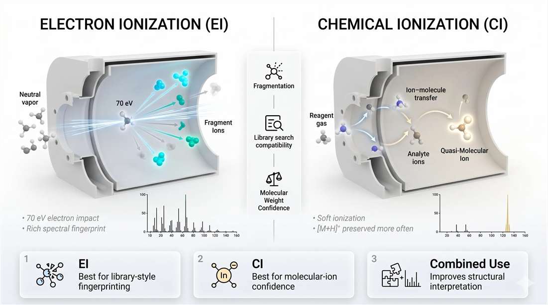
Figure 5. EI versus CI in GC-MS. EI emphasizes fragmentation and generates rich library-searchable spectral fingerprints. CI reduces fragmentation and improves preservation of molecular-ion-related signal. In practice, EI is often preferred for spectral matching, while CI adds value when molecular-weight confirmation is the limiting need.
When hard ionization is the right answer
EI is the right tool when fragmentation is an asset. That includes routine library-based identification, established compound panels, and workflows where fragment-pattern comparison is the fastest route to a confident result.
This is one reason EI fits so well into untargeted metabolomics. In these studies, a fragment-rich spectrum often improves the ability to separate plausible candidates. The same logic applies when GC-based metabolite evidence needs to align with broader pathway or systems-level interpretation in integrated proteomics and metabolomics analysis. If the fragment logic is weak, the biological interpretation built on top of it becomes weaker too.
EI is also valuable when the chemical space is already represented well in libraries. In those cases, fragmentation is not noise. It is the main language of identification.
When soft ionization becomes the stronger choice
CI becomes more useful when the missing information is not fragmentation but intact-mass confidence. If EI produces many informative fragments but no strong molecular ion, the result may still be incomplete. CI can close that gap.
This is especially helpful for compounds that fragment too easily, for analytes with close structural analogs, and for workflows where molecular weight is needed to anchor interpretation before any downstream filtering begins. In these settings, a softer ionization route improves confidence by preserving information that EI may sacrifice.
A mature GC-MS workflow therefore does not treat ionization mode as a fixed default. It treats ionization mode as part of the identification strategy. That mindset is increasingly important in projects that combine analytical chemistry with downstream bioinformatics for metabolomics, because the quality of the original identity call determines how credible the later biological statistics will be.
GC-FID vs GC-MS: Choosing the Detector by Analytical Intent
For many buyers, the harder detector decision is not EI versus CI. It is whether the method needs mass spectrometry at all.
This question is often answered poorly because GC-MS sounds more advanced and therefore seems automatically better. That is not always true. Detector choice should follow analytical intent, not instrument prestige.
FID and MS solve different problems.
FID is strong when the method needs stable, wide-range quantitation for organic analytes that respond well in a flame ionization environment. GC-MS is stronger when the method must identify unknowns, distinguish real analyte signal from matrix background, or provide structural evidence rather than only a concentration value.
What FID does well
FID is often underestimated because it is simple. But simplicity is one of its strengths. In routine settings, FID can offer:
- strong linear dynamic range
- reliable peak-area response
- robust routine performance
- relatively straightforward data handling
- excellent fit for defined analyte panels
That makes it attractive for controlled assays, routine QC, and workflows where compound identity is already well established and the primary task is consistent quantitation.
This is one reason FID still has a clear place in applied service environments. If the analytical question is focused and the target compounds are known, detector simplicity can be an advantage rather than a limitation.
What GC-MS does better
GC-MS earns its place when identity becomes part of the deliverable. It is stronger in:
- unknown identification
- matrix discrimination
- confirmatory analysis
- isomer-sensitive interpretation
- structurally informed screening
In complex biological or environmental matrices, a peak is not always just a peak. Co-elution, background contamination, and partial overlap can all distort what looks acceptable by chromatographic review alone. GC-MS adds another layer of scrutiny. It allows the analyst to ask whether the signal matches the expected mass pattern, whether interferences are present, and whether the feature is chemically plausible.
That is why GC-MS is so valuable in metabolomics service, targeted metabolomics, short-chain fatty acid analysis, and organic acid analysis, where quantitation and identity confidence often need to coexist.
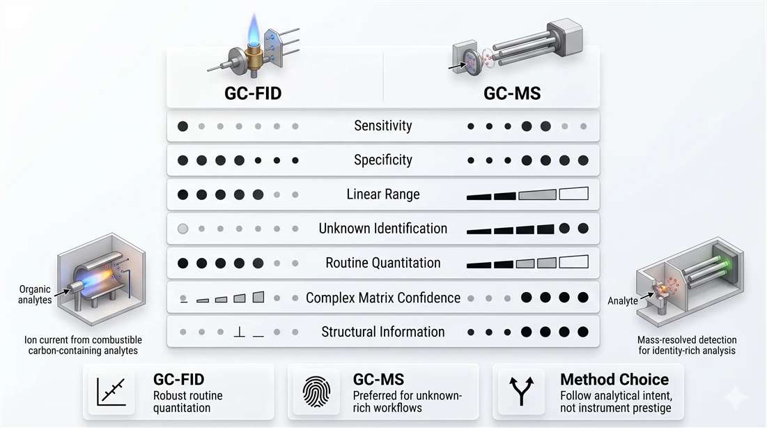
Figure 6. GC-FID versus GC-MS as a method-selection decision matrix. GC-FID is often preferred for robust routine quantitation with wide linear range and simpler workflows. GC-MS is preferred when specificity, unknown identification, matrix confidence, or structural interpretation are central to the analytical objective.
Comparison Table: GC-FID vs GC-MS
| Metric | GC-FID | GC-MS |
| Sensitivity | Strong for many carbon-containing analytes | Strong, but depends on ionization mode and acquisition strategy |
| Specificity | Limited structural specificity | High specificity through mass-resolved detection |
| Linear Range | Typically very wide | Strong, but often more method-dependent |
| Suitability for Routine Quantitation | Excellent | Very good, especially when identity confirmation is also needed |
| Suitability for Unknown Identification | Weak | Excellent |
| Matrix Confidence | Moderate | High |
| Structural Information | Minimal | High |
| Data Complexity | Lower | Higher |
| Best Use Case | Defined analyte panels and routine QC | Unknown-rich, confirmatory, and structurally driven workflows |
A better detector decision rule
The simplest way to choose between FID and GC-MS is to ask one direct question:
Is the final deliverable mainly a number, or is it a number plus identity confidence?
If the answer is mainly a number, FID may be the most efficient solution.
If the answer includes structural confirmation, unknown annotation, or matrix-specific specificity, GC-MS is usually the stronger choice.
This becomes even more important when the project extends into downstream data layers such as multivariate analysis service or integrated metabolomics and microbiomics analysis. Weak structural confidence at the detector stage will weaken every later conclusion built on that data matrix.
A Practical Method-Development Sequence for Precision GC
At this point, the logic of precision gas chromatography becomes clear. High-resolution volatile analysis does not come from one good setting. It comes from a sequence of aligned decisions.
A strong method usually follows this order.
1. Define the analytical endpoint first
Start by deciding whether the method needs routine quantitation, broad screening, unknown identification, or confirmation-grade structural evidence. This determines whether FID, EI-MS, CI-MS, or a combined strategy is the right endpoint.
A method designed for targeted metabolomics should not be structured the same way as a workflow built for unknown metabolite identification. The endpoint changes everything upstream.
2. Choose phase chemistry for selectivity
Select the stationary phase based on the interaction differences that need to be amplified. Do not reduce this decision to a simple polarity label. Think in terms of which compound classes must be separated most clearly.
3. Choose film thickness for the volatility window
Set (d_f) according to the part of the analyte range that needs the most control. If very volatile compounds are failing early, retention support may matter more than speed. If the method is already broad and slow, a thinner film may reduce transfer penalty.
4. Tune carrier-gas velocity around the real column physics
Once phase and film are set, optimize linear velocity. Do not do this first. Velocity must fit the actual transfer behavior of the column configuration that will be used in production.
5. Validate inlet transfer before blaming the column
Check liner volume, vapor expansion, split strategy, and discrimination risk. If the sample enters the column badly, no downstream optimization can fully rescue the method.
This is a critical checkpoint in workflows such as short-chain fatty acid analysis and organic acid analysis, where early-band integrity often determines whether the assay will be robust at all.
6. Add retention-index logic where identification matters
For unknown-rich methods, retention time alone is not enough. RI adds a more transferable retention coordinate and strengthens annotation when paired with spectral evidence.
This is especially useful in GC-MS/MS untargeted metabolomics and untargeted metabolomics, where feature confidence benefits from every orthogonal layer of support.
7. Match ionization mode to the uncertainty that remains
If fragment pattern is the main need, EI is usually the best path. If molecular-ion preservation is the missing piece, CI may add more value. If both questions matter, use both modes strategically.
That sequence is what turns GC from an instrument into a controlled analytical system.
Conclusion
Gas chromatography becomes far more powerful when it is understood as a method-development discipline rather than a standard instrument category. The best GC methods do not emerge from isolated adjustments. They emerge from aligned control of kinetics, selectivity, transfer, and detection.
The Van Deemter equation explains why efficiency has a bounded operating window. Stationary-phase chemistry explains why compounds that look similar on paper may separate very differently in practice. Film thickness explains why volatile retention and transfer burden are always linked. Inlet physics explains why a bad band can be created before the column ever has a chance to perform. And detector choice explains whether the final output is merely quantitative or truly informative.
For advanced analytical buyers, that distinction matters. A credible GC workflow is not defined by one impressive instrument specification. It is defined by whether the method can hold together from injection to identification. That is the difference between a chromatogram that looks good and a workflow that produces results strong enough to support real scientific decisions.
In service settings, that same logic determines whether the platform can scale into broader interpretation. Strong GC data is not only useful on its own. It also strengthens downstream bioinformatics for metabolomics, supports more stable multivariate analysis service, and integrates more cleanly into packages such as integrated proteomics and metabolomics analysis. Precision GC, in other words, is not just about separation. It is about building analytical confidence that survives the rest of the workflow.
FAQ
1. What is the most common mistake in GC method development?
The most common mistake is optimizing flow or oven conditions before the stationary phase and film thickness have been matched to the analyte chemistry and volatility range. This often produces a method that looks acceptable but remains fragile.
2. Does lower plate height always mean better separation?
No. Lower plate height improves efficiency, but resolution also depends on retention and selectivity. A method can produce narrow peaks and still fail if the analytes remain too close together.
3. When should I use a thicker GC film?
A thicker film is most useful when highly volatile analytes elute too early, when front-end retention is weak, or when phase capacity needs to increase. The tradeoff is more mass-transfer burden and a higher risk of peak broadening.
4. Why are my early peaks distorted even though the column seems fine?
The problem may be at the inlet, not in the column. Backflash, poor vapor containment, or unsuitable transfer conditions can distort the band before chromatography begins.
5. Is EI always better than CI for GC-MS?
No. EI is usually better for fragmentation-rich library matching. CI is more useful when molecular-ion preservation or molecular-weight confidence is the main need.
6. When is GC-FID better than GC-MS?
GC-FID is often better for routine quantitation of known compounds when wide linear range, robustness, and simpler data handling matter more than structural interpretation.
7. Why is Kovats retention index still important?
Because retention time alone is method-specific. RI gives a more transferable retention coordinate and becomes much more valuable when paired with spectral evidence.
8. Can one GC method be ideal for both highly volatile and semi-volatile compounds?
Sometimes, but it is difficult. The same film thickness and operating conditions that improve the front end may reduce efficiency or extend run time for later compounds. Broad-boiling-range methods usually require deliberate compromise.
References
- van Deemter JJ, Zuiderweg FJ, Klinkenberg A. Longitudinal diffusion and resistance to mass transfer as causes of nonideality in chromatography. Chemical Engineering Science. 1956;5(6):271-289. DOI:10.1016/0009-2509(56)80003-1
- Kováts E. Gas-chromatographische Charakterisierung organischer Verbindungen. Teil 1: Retentionsindices aliphatischer Halogenide, Alkohole, Aldehyde und Ketone. Helvetica Chimica Acta. 1958;41(7):1915-1932. DOI:10.1002/hlca.19580410703
- Traitler H. Recent advances in capillary gas chromatography applied to lipid analysis. Progress in Lipid Research. 1987;26(4):257-280. DOI:10.1016/0163-7827(87)90001-4
- Zellner BD, Bicchi C, Dugo P, Rubiolo P, Dugo G, Mondello L. Linear retention indices in gas chromatographic analysis: a review. Flavour and Fragrance Journal. 2008;23(5):297-314. DOI:10.1002/ffj.1887
Related Services
- Unknown Metabolites Identification
- Xenobiotic Metabolites Analysis
- Metabolomics Service
- Targeted Metabolomics
- Short Chain Fatty Acids Analysis
- Organic Acid Analysis Solution
- Fatty Acids Metabolomics Service
- Bioinformatics for Metabolomics
- Multivariate Analysis Service
*For Research Use Only. Not for use in diagnostic procedures.
More Articles
- What is Phytosterols
Learn about phytosterols - plant-based compounds that have cholesterol-lowering properties and potential health benefits. - Preparation and Development of GC Capillary Column
Learn about the preparation and development of GC capillary columns, an important component in gas chromatography analysis. - What Is Acyl-CoAs Metabolism
Discover the vital role of Acyl-CoAs in cellular metabolism, including fatty acid oxidation, synthesis, cholesterol metabolism, and ketogenesis. Learn how Creative Proteomics' innovative Acyl-CoAs assay can advance your research.